Research Article Volume 11 Issue 1
Reliability estimation of type-II generalized loglogistic distribution
SVSVSV Prasad,1 Gadde Srinivasa Rao,2
K. Rosaiah1
1Department of Statistics, Acharya Nagarjuna University, India
2Department of Mathematics and Statistics, The University of Dodoma, Tanzania
Correspondence: Gadde Srinivasa Rao, Department of Mathematics and Statistics, The University of Dodoma, Dodoma, P.O. Box: 259, Tanzania
Received: December 20, 2021 | Published: February 28, 2022
Citation: Prasad SVSVSV, Rao GS, Rosaiah K. Reliability estimation of type-II generalized log-logistic distribution. Biom Biostat Int J. 2022;11(1):36-46. DOI: 10.15406/bbij.2022.11.00352
Download PDF
Abstract
In this article, a lifetime distribution named as Type-II generalized log-logistic distribution (TGLLD) is considered and its failure rate of products with different shape parameters used to find out ageing criteria. An attempt has been made to derive the statistical and reliability properties of TGLLD. Parameters are evaluated using maximum likelihood estimation and obtained the reliability of the distribution. A simulation study also conducted to know the performance of the estimators. The estimates obtained are validated with the use of live data.
Keywords: type-ii generalized log-logistic distribution, reliability function, hazard rate, reverse hazard rate, moments, maximum likelihood estimation
MATHEMATICS SUBJECT CLASSIFICATION: 62F10; 62F15; 62N05
Introduction
Over a period of time, statistical literature witnessed the origin of many continuous univariate distributions. However, in the present era, these distributions are extended by introducing the additional parameters in order to cater the requirements from different areas such as lifetime analysis, finance, engineering industries, insurance etc. The present distribution dealt in this article is one such distribution introduced by Rosaiah et al.1 When a distribution is introduced, one may keen to know the behavior for its characterization. The same can be achieved by finding its statistical properties viz., mean, median, mode, variance, quantiles, moments, cumulants, order statistics, ML estimates, confidence intervals etc. Distinguished authors have made their efforts in estimating such properties for different distributions viz. Balakrishnan2,3 for half logistic and generalized logistic, Mudholkar and Srivastava4 Mudholkar5 for exponentiated Weibull, Gupta et al.6 for log-logistic, Nadarajah7 for exponentiated Gumbel, Nadarajah and Gupta8 for exponentiated gamma, Abouammoh and Alshingiti9 for inverted exponential distribution, Rosaiah et. al.10 for odds exponential log logistic Distribution and many more.
Log-logistic distribution (LLD) has proven its importance in quality control, mainly in analyzing the lifetime data. Many authors have made their contribution in developing the various features of this distribution by creating some extensions to the original distribution, Type-II generalized log-logistic distribution (TGLLD) is one such distribution. In this article an effort to derive mathematical properties of TGLLD. The rest of the article is organized as follows. In Section 2, the cumulative distribution function, probability density function, reliability function and hazard function of TGLLD are given. Also, the key properties, moments of TGLLD and ith order statistic are obtained. In Section 3, ML estimators, asymptotic confidence intervals are derived. Fitting reliability data, computation of ML estimates, statistics such as -2logL, AIC and BIC are presented in section 4. Lastly in Section 5, the concluding remarks are given.
Type-II generalized log logistic distribution
Log-logistic distribution (LLD) has proven its importance in quality control. Different authors developed properties and types of acceptance sampling plans for LLD viz., Ashkar and Mahdi.11 The cumulative distribution function (CDF) of the log-logistic distribution (LLD) is
(1)
Since the practical pertinence of generalized log-logistic distribution (GLLD) in diverse sectors, various authors have paid their attention in developing some extensions for effective and wide use of log-logistic distribution. One such extension to this distribution named as Type-II generalized log-logistic distribution (TGLLD) introduced by Rosaiah et al.,1 its cumulative distribution function (cdf) is
(2)
It may be noted that the distribution given in (2) is defined through the reliability oriented generalization of log-logistic distribution. In short, we call this as the Type-II generalized log-logistic distribution [Type-I generalized (exponentiated) log-logistic distribution is dealt by Rosaiah et al.12 The corresponding probability density function (PDF) is given by
(3)
where σ is the scale parameter, λ and θ are shape parameters.
Rao et al.13,14 developed the reliability test plans for this distribution. The reliability function and hazard (failure rate) function of type-II generalized log-logistic distribution are respectively given by
(4)
(5)
The three-parameter TGLLD will be denoted by TGLLD
. If
, then Eq. (3) becomes log-logistic distribution and if
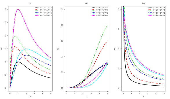
=1 then TGLLD becomes reduced to Pareto type-II distribution. Figures 1-4 depicted that the PDF, CDF, reliability function and hazard function curves of TGLLD for various parametric combinations.
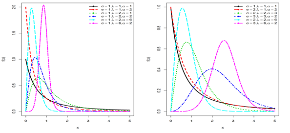
Figure 1 The probability density function of TGLLD for different
and
at
.

Figure 2 The cumulative density function of TGLLD for different
and
at
.
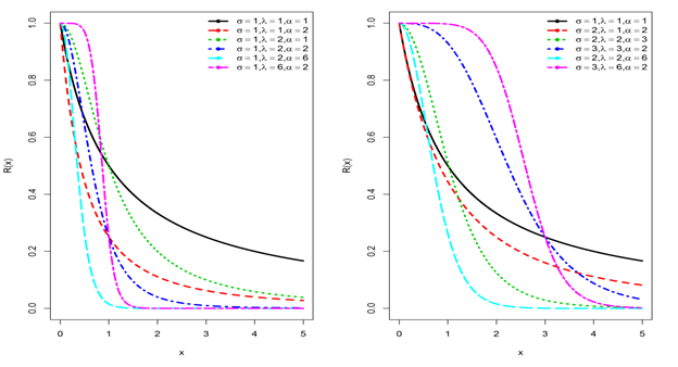
Figure 3 The reliability function of TGLLD for different
and
at
.

Figure 4 The hazard function of TGLLD for different
and
at
. (a) Upside-down bathtub
(b) Increasing (c) Decreasing.
Properties of the TGLLD
Limits of the distribution function
Reverse hazard function of a non-negative random variable is
(6)
The odd function of a random variable can be derived from
(7)
Mean of TGLLD is derived as
(8)
Percentile and median
The
percentile of a random variable T is denoted by
and is defined as
where
If
is unique for each
is an inverse function, then
Percentile,
(9)
Quantile function
Median (M) (50th percentiles) is
(10)
Mode of TGLLD is obtained as the value of x for which
and
.
Hence mode is the solution of the non-linear equation
Moments of TGLLD
Moments are the useful tools which can be used to derive the key features of the distribution. Here we tried to derive
moment of the random variable T, where
.
The
moment of T is denoted by
and is defined as
(11)
Variance =
Mean, median, skewness and kurtosis of TGLLD for various combinations of
,
and
are given in Table 1.
|
λ
|
θ
|
σ
|
Mean
|
Median
|
Skewness
|
Kurtosis
|
|
1.5
|
1.5
|
1
|
1.1498
|
0.7014
|
4.0543
|
3.0912
|
|
2.5
|
2.5
|
1
|
0.6985
|
0.6336
|
2.5365
|
9.9632
|
|
3
|
3
|
1
|
0.6718
|
0.6382
|
0.8453
|
5.1318
|
|
3.5
|
3.5
|
1
|
0.6657
|
0.648
|
0.3195
|
3.8556
|
|
4
|
4
|
1
|
0.6682
|
0.6595
|
0.112
|
3.3635
|
|
4.5
|
4.5
|
1
|
0.6744
|
0.6714
|
0.0283
|
3.1535
|
|
5
|
5
|
1
|
0.6824
|
0.6831
|
0.0016
|
3.07
|
|
5.5
|
5.5
|
1
|
0.6911
|
0.6942
|
0.0039
|
3.0504
|
|
6
|
6
|
1
|
0.6999
|
0.7047
|
0.0215
|
3.0653
|
|
2
|
3
|
2
|
1.1781
|
1.0196
|
3.6429
|
12.4635
|
|
3
|
2
|
3
|
2.4184
|
2.2363
|
2.5253
|
10.8095
|
|
2
|
6
|
2
|
0.7731
|
0.6999
|
1.1978
|
5.1176
|
|
6
|
2
|
3
|
2.618
|
2.5902
|
0.1888
|
4.1057
|
Table 1 Mean, Median, Skewness and Kurtosis of TGLLD for various combinations of
Moment Generating function (MGF) is given by
(12)
Characteristic Function is given by
(13)
Cumulative Generating function is defined by
(14)
Order statistics of TGLLD
Let
denotes the order statistics obtained from a random sample of size n drawn from TGLLD
The probability density function of ith order statistic is given by
(15)
Since
for
, then using binomial expansion
(16)
Then
(17)
Now take
Hence
(18)
The distribution function of ith order statistic T(i) is
, using (16), it can be expressed as
(19)
Distribution function of first order statistic T(1) is
(20)
Distribution function of nth order statistic T(n) is
(21)
Parameter estimation and inference
For estimating the parameters of
, we considered two known methods viz., maximum likelihood method of estimation and least square method. It is observed that the estimates obtained from both methods for the unknown parameters cannot be expressed in closed form and hence the estimates are obtained using simulation study.
Maximum likelihood estimators (MLEs)
Let
be a random sample of size n drawn from TGLLD
, then likelihood function L of the sample is
The log-likelihood function is
(22)
The MLE’s of
and
are obtained as
(23)
(24)
(25)
Using Eq. (25) in Eqs. (23) and (24) we get two equations in terms of
, these equations cannot be solved analytically, so they need to be solved numerically. Iterative techniques can be applied for obtaining the estimators of the parameters. Let
are ML estimates of the parameters
respectively. Using invariance property of the MLE, the MLE of reliability function can be obtained by
(26)
Asymptotic confidence interval
Here, an attempt has been made to derive the asymptotic confidence intervals of the unknown parameters
and
. Using large sample approach and assume that the MLE’s of
are approximately multivariate normal with mean
and Variance-covariance matrix
, where
is observed information matrix which is defined as
=
(27)
Now, the second order partial derivatives of the parameters given in
are
(28)
(29)
(30)
(31)
(32)
(33)
(33)
(34)
(35)
The Asymptotic
confidence interval of
are
,
and
respectively, where
is the upper
percentile of the standard normal distribution.
To obtain the asymptotic confidence interval for
, we proceed as follows.
The asymptotic variance of the MLEs are given by
(36)
(37)
(38)
Now
(39)
(40)
(41)
The asymptotic variance (A V) of an estimate of
which is a function of parameter estimates (say)
is given by Rao15
(42)
Thus the asymptotic variance of
can be obtained after substituting equations (36) to (41) in equation (42), which will be analytically solved thereafter.
Samples are generated at varying sizes n = 20, 30, 40, 50 and 100 for different assumed values of shape parameters λ and θ when
. MLEs, mean square error (MSE) and bias of λ when θ is assumed as 1.5, 2 and 2.5 are presented in Table 2. Similarly MLEs, MSE and bias of θ when λ is assumed as 1.5, 2 and 2.5 are presented in Table 3. Table 4 represents the values of MLEs, mean square error (MSE) and bias of reliability function (R) for the parametric combinations of (λ, θ) = (1.5, 1.5), (1.5, 2), (2, 1.5), (2, 2), (2, 2.5), (2.5, 2) and (2.5, 2.5).
| |
n = 20
|
n = 30
|
n = 40
|
n = 50
|
n = 100
|
|
(θ = 2)
|
|
|
|
|
|
|
|
1.5000
|
1.5000
|
1.5000
|
1.5000
|
1.5000
|
|
|
1.5968
|
1.5625
|
1.5471
|
1.5372
|
1.5182
|
|
Bias
|
0.0968
|
0.0625
|
0.0471
|
0.0372
|
0.0182
|
|
MSE
|
0.0991
|
0.0576
|
0.0410
|
0.0319
|
0.0148
|
|
(θ =1.5)
|
|
|
|
|
|
|
|
2.0000
|
2.0000
|
2.0000
|
2.0000
|
2.0000
|
|
|
2.1374
|
2.0885
|
2.0668
|
2.0527
|
2.0257
|
|
Bias
|
0.1374
|
0.0885
|
0.0668
|
0.0527
|
0.0257
|
|
MSE
|
0.2027
|
0.1166
|
0.0828
|
0.0641
|
0.0297
|
|
(θ = 2)
|
|
|
|
|
|
|
|
2.0000
|
2.0000
|
2.0000
|
2.0000
|
2.0000
|
|
|
2.1290
|
2.0833
|
2.0628
|
2.0496
|
2.0242
|
|
Bias
|
0.1290
|
0.0833
|
0.0628
|
0.0496
|
0.0242
|
|
MSE
|
0.1761
|
0.1025
|
0.0730
|
0.0566
|
0.0263
|
|
(θ =2.5)
|
|
|
|
|
|
|
|
2.0000
|
2.0000
|
2.0000
|
2.0000
|
2.0000
|
|
|
2.1264
|
2.0816
|
2.0614
|
2.0485
|
2.0237
|
|
Bias
|
0.1264
|
0.0816
|
0.0614
|
0.0485
|
0.0237
|
|
MSE
|
0.1648
|
0.0959
|
0.0682
|
0.0530
|
0.0246
|
|
(θ =2.5)
|
|
|
|
|
|
|
|
2.5000
|
2.5000
|
2.5000
|
2.5000
|
2.5000
|
|
|
2.6580
|
2.6019
|
2.5768
|
2.5606
|
2.5296
|
|
Bias
|
0.1580
|
0.1019
|
0.0768
|
0.0606
|
0.0296
|
|
MSE
|
0.2574
|
0.1499
|
0.1066
|
0.0828
|
0.0385
|
Table 2 MLE of λ when σ = 30 for TGLLD
| |
n = 20
|
n = 30
|
n = 40
|
n = 50
|
n =100
|
|
(λ = 1.5)
|
|
|
|
|
|
|
|
1.5000
|
1.5000
|
1.5000
|
1.5000
|
1.5000
|
|
|
1.5771
|
1.5487
|
1.5347
|
1.5279
|
1.5133
|
|
Bias
|
0.0771
|
0.0487
|
0.0347
|
0.0279
|
0.0133
|
|
MSE
|
0.1664
|
0.0962
|
0.0679
|
0.0524
|
0.0246
|
|
(λ = 1.5)
|
|
|
|
|
|
|
|
2.0000
|
2.0000
|
2.0000
|
2.0000
|
2.0000
|
|
|
2.1380
|
2.0863
|
2.0619
|
2.0494
|
2.0235
|
|
Bias
|
0.1380
|
0.0863
|
0.0619
|
0.0494
|
0.0235
|
|
MSE
|
0.3282
|
0.1794
|
0.1236
|
0.0940
|
0.0433
|
|
(λ = 2)
|
|
|
|
|
|
|
|
2.0000
|
2.0000
|
2.0000
|
2.0000
|
2.0000
|
|
|
2.1380
|
2.0863
|
2.0619
|
2.0494
|
2.0235
|
|
Bias
|
0.1380
|
0.0863
|
0.0619
|
0.0494
|
0.0235
|
|
MSE
|
0.3282
|
0.1794
|
0.1236
|
0.0940
|
0.0433
|
|
(λ = 2.5)
|
|
|
|
|
|
|
|
2.0000
|
2.0000
|
2.0000
|
2.0000
|
2.0000
|
|
|
2.1380
|
2.0863
|
2.0619
|
2.0494
|
2.0235
|
|
Bias
|
0.1380
|
0.0863
|
0.0619
|
0.0494
|
0.0235
|
|
MSE
|
0.3282
|
0.1794
|
0.1236
|
0.0940
|
0.0433
|
|
(λ = 2)
|
|
|
|
|
|
|
|
2.5000
|
2.5000
|
2.5000
|
2.5000
|
2.5000
|
|
|
2.7155
|
2.6334
|
2.5959
|
2.5761
|
2.5361
|
|
Bias
|
0.2155
|
0.1334
|
0.0959
|
0.0761
|
0.0361
|
|
MSE
|
0.6020
|
0.3118
|
0.2096
|
0.1575
|
0.0708
|
|
(λ = 2.5)
|
|
|
|
|
|
|
|
2.5000
|
2.5000
|
2.5000
|
2.5000
|
2.5000
|
|
|
2.7155
|
2.6334
|
2.5959
|
2.5761
|
2.5361
|
|
Bias
|
0.2155
|
0.1334
|
0.0959
|
0.0761
|
0.0361
|
|
MSE
|
0.6020
|
0.3118
|
0.2096
|
0.1575
|
0.0708
|
Table 3 MLE of θ when σ = 30 for TGLLD
| |
n = 20
|
n = 30
|
n = 40
|
n = 50
|
n =100
|
|
(λ = 1.5, θ = 1.5)
|
|
|
|
|
|
|
|
0.9977
|
0.9977
|
0.9977
|
0.9977
|
0.9977
|
|
Bias
|
-0.0009
|
-0.0006
|
-0.0004
|
-0.0004
|
-0.0002
|
|
MSE
|
0.0005
|
0.0004
|
0.0004
|
0.0003
|
0.0002
|
|
(λ = 1.5, θ = 2)
|
|
|
|
|
|
|
|
0.9978
|
0.9978
|
0.9978
|
0.9978
|
0.9978
|
|
Bias
|
-0.0008
|
-0.0005
|
-0.0004
|
-0.0003
|
-0.0002
|
|
MSE
|
0.0008
|
0.0007
|
0.0007
|
0.0004
|
0.0002
|
|
(λ = 2, θ = 1.5)
|
|
|
|
|
|
|
|
0.9996
|
0.9996
|
0.9996
|
0.9996
|
0.9996
|
|
Bias
|
0.0003
|
-0.0002
|
-0.0002
|
-0.0001
|
-0.0001
|
|
MSE
|
0.0008
|
0.0006
|
0.0005
|
0.0003
|
0.0002
|
|
(λ = 2, θ = 2)
|
|
|
|
|
|
|
|
0.9996
|
0.9996
|
0.9996
|
0.9996
|
0.9996
|
|
Bias
|
-0.0003
|
-0.0002
|
-0.0001
|
-0.0001
|
-0.0001
|
|
MSE
|
0.0009
|
0.0007
|
0.0006
|
0.0005
|
0.0003
|
|
(λ = 2, θ = 2.5)
|
|
|
|
|
|
|
|
0.9996
|
0.9996
|
0.9996
|
0.9996
|
0.9996
|
|
Bias
|
-0.0003
|
-0.0002
|
-0.0001
|
-0.0001
|
0.0000
|
|
MSE
|
0.0009
|
0.0008
|
0.0007
|
0.0006
|
0.0003
|
|
(λ = 2.5, θ = 2)
|
|
|
|
|
|
|
|
0.9999
|
0.9999
|
0.9999
|
0.9999
|
0.9999
|
|
Bias
|
-0.0001
|
-0.0001
|
0.0000
|
0.0000
|
0.0000
|
|
MSE
|
0.0009
|
0.0008
|
0.0006
|
0.0005
|
0.0003
|
|
(λ = 2.5, θ = 2.5)
|
|
|
|
|
|
|
|
0.9999
|
0.9999
|
0.9999
|
0.9999
|
0.9999
|
|
Bias
|
-0.0001
|
-0.0001
|
0.0001
|
0.0001
|
0.0002
|
|
MSE
|
0.0009
|
0.0008
|
0.0007
|
0.0006
|
0.0004
|
Table 4 MLE of R when σ = 30 for TGLLD
It can be seen from Tables 2 and 3, the bias and MSE of both λ and θ decrease as the sample size increases. This reflects the asymptotic consistency property of the MLEs. From Table 2, when the parameter λ increases the concerned bias and MSE are also observed as increases and the rate of this increment is high at smaller sample sizes especially till sample size n reaches 50. Similar pattern noticed for the parameter θ from Table 3.
From Table 4, it is observed that when both parameters are increases, the
resulted more accurate values and the absolute bias decreases as the sample size increases. Also mse of
observed as very small values. From Table 5 we noticed that average length of 95% confidence interval is decreases as sample size and parametric values are increases furthermore the coverage probabilities for λ and θ are very close to 95% that we expected. The results shows that estimation and confidence limits of shape parameter λ and θ are performed well using maximum likelihood estimation.
|
n
|
λ
|
θ
|
Average length
|
Coverage Probability
|
|
λ
|
θ
|
λ
|
θ
|
|
20
|
2.0
|
1.5
|
1.5510
|
1.4140
|
0.9410
|
0.9373
|
|
30
|
2.0
|
1.5
|
1.2360
|
1.1310
|
0.9455
|
0.9423
|
|
40
|
2.0
|
1.5
|
1.0590
|
0.9701
|
0.9461
|
0.9433
|
|
50
|
2.0
|
1.5
|
0.9403
|
0.8634
|
0.9471
|
0.9449
|
|
100
|
2.0
|
1.5
|
0.6559
|
0.6043
|
0.9474
|
0.9484
|
|
20
|
1.5
|
1.5
|
1.1640
|
1.4140
|
0.9410
|
0.9373
|
|
30
|
1.5
|
1.5
|
0.9270
|
1.1310
|
0.9456
|
0.9423
|
|
40
|
1.5
|
1.5
|
0.7942
|
0.9701
|
0.9461
|
0.9433
|
|
50
|
1.5
|
1.5
|
0.7052
|
0.8634
|
0.9470
|
0.9449
|
|
100
|
1.5
|
1.5
|
0.4919
|
0.6043
|
0.9474
|
0.9485
|
|
20
|
2.0
|
2.0
|
1.4550
|
1.9070
|
0.9406
|
0.9375
|
|
30
|
2.0
|
2.0
|
1.1620
|
1.5080
|
0.9453
|
0.9422
|
|
40
|
2.0
|
2.0
|
0.9965
|
1.2870
|
0.9463
|
0.9434
|
|
50
|
2.0
|
2.0
|
0.8855
|
1.1420
|
0.9471
|
0.9445
|
|
100
|
2.0
|
2.0
|
0.6185
|
0.7951
|
0.9479
|
0.9476
|
|
20
|
2.5
|
2.0
|
1.8180
|
1.9070
|
0.9406
|
0.9375
|
|
30
|
2.5
|
2.0
|
1.4520
|
1.5080
|
0.9453
|
0.9422
|
|
40
|
2.5
|
2.0
|
1.2460
|
1.2870
|
0.9463
|
0.9434
|
|
50
|
2.5
|
2.0
|
1.1070
|
1.1420
|
0.9471
|
0.9445
|
|
100
|
2.5
|
2.0
|
0.7732
|
0.7951
|
0.9479
|
0.9476
|
|
20
|
2.5
|
2.5
|
1.7570
|
2.4850
|
0.9403
|
0.9367
|
|
30
|
2.5
|
2.5
|
1.4040
|
1.9410
|
0.9449
|
0.9418
|
|
40
|
2.5
|
2.5
|
1.2040
|
1.6480
|
0.9461
|
0.9440
|
|
50
|
2.5
|
2.5
|
1.0700
|
1.4580
|
0.9470
|
0.9432
|
|
100
|
2.5
|
2.5
|
0.7476
|
1.0100
|
0.9481
|
0.9482
|
|
20
|
1.5
|
2.0
|
1.0910
|
1.9070
|
0.9406
|
0.9375
|
|
30
|
1.5
|
2.0
|
0.8715
|
1.5080
|
0.9453
|
0.9422
|
|
40
|
1.5
|
2.0
|
0.7474
|
1.2870
|
0.9463
|
0.9434
|
|
50
|
1.5
|
2.0
|
0.6641
|
1.1420
|
0.9471
|
0.9445
|
|
100
|
1.5
|
2.0
|
0.4639
|
0.7951
|
0.9479
|
0.9476
|
|
20
|
2.0
|
2.5
|
1.4060
|
2.4850
|
0.9403
|
0.9367
|
|
30
|
2.0
|
2.5
|
1.1230
|
1.9410
|
0.9449
|
0.9418
|
|
40
|
2.0
|
2.5
|
0.9633
|
1.6480
|
0.9461
|
0.9440
|
|
50
|
2.0
|
2.5
|
0.8560
|
1.4580
|
0.9471
|
0.9432
|
|
100
|
2.0
|
2.5
|
0.5980
|
1.0100
|
0.9482
|
0.9482
|
Table 5 Average length and coverage probability of
and
when
=30
Fitting reliability data
In this section, we considered a real data set to compare the ML estimates of TGLLD given in (3), with the log-logistic (LL), McDonald log-logistic (McLL) studied by Tahir et al.,16 beta log-logistic (BeLL) by Lemonte,17 Kumaraswamy log-logistic (KwLL) discussed by de Santana et al.,18 Marshal-Olkin log-logistic (MoLL) developed by Gui.19 The corresponding densities functions of the above distributions are reproduced below.
LL:
McLL:
BeLL:
KwLL:
MoLL:
We will be considering the single fibers of 20mm in gauge length, with sample sizes n = 69 respectively. For easy reference, this data is presented below.
1.312, 1.314, 1.479, 1.552, 1.700, 1.803, 1.861, 1.865, 1.944, 1.958, 1.966, 1.997, 2.006, 2.021, 2.027, 2.055, 2.063, 2.098, 2.140, 2.179, 2.224, 2.240, 2.253, 2.270, 2.272, 2.274, 2.301, 2.301, 2.359, 2.382, 2.382, 2.426, 2.434, 2.435, 2.478, 2.490, 2.511, 2.514, 2.535, 2.554, 2.566, 2.570, 2.586, 2.629, 2.633, 2.642, 2.648, 2.684, 2.697, 2.726, 2.770, 2.773, 2.800, 2.809, 2.818, 2.821, 2.848, 2.880, 2.954, 3.012, 3.067, 3.084, 3.090, 3.096, 3.128, 3.233, 3.433, 3.585, 3.585.
Table 6 describes the fitted data of MLEs of the unknown parameters of different log-logistic distributions, it is observed that TGLLD throws better results and found more suitable in analyzing the data. Plots of empirical and fitted PDFs drawn for the observed data are shown in Figure 5.
|
Model
|
Estimates
|
-2logL
|
AIC
|
BIC
|
|
TGLLD (λ, σ, θ)
|
6.509 (1.0967)
|
3.119 (0.6536)
|
3.595 (3.5802)
|
|
|
97.84
|
103.8
|
110.5
|
|
LL (λ, σ)
|
8.484 (0.8531)
|
2.431 (0.0598)
|
|
|
|
101.56
|
105.6
|
110
|
|
McLL (λ, σ, a, b, c)
|
5.493 (18.802)
|
2.655 (0.07716)
|
1.282
(5.6039)
|
4.353 (30.5138)
|
4.42 (11.27)
|
97.82
|
107.8
|
119
|
|
BeLL (λ, σ, a, b)
|
5.624 (5.441)
|
3.298
(1.755)
|
1.227
(1.617)
|
5.129 (14.521)
|
|
97.78
|
105.8
|
114.7
|
|
KwLL (λ, σ, a, b)
|
4.002 (10.091)
|
3.436
(1.811)
|
1.778
(5.328)
|
11.064 (70.15)
|
|
97.74
|
105.7
|
114.7
|
|
MoLL (λ, σ, α)
|
8.484 (0.8532)
|
2.055 (2.3428)
|
4.162 (40.2466)
|
|
|
101.56
|
107.6
|
114.3
|
Table 6 The MLEs (SEs in parentheses) and statistics of the distribution parameters
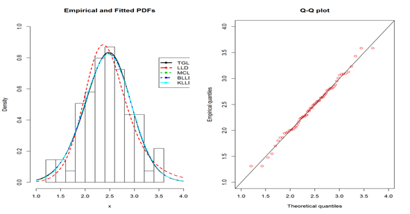
Figure 5 Fitted PDFs of different log-logistic distributions along with TGLLD and Q-Q plot for the observed data.
Conclusion
In this article, a lifetime distribution named as Type-II generalized log-logistic distribution (TGLLD) is considered. We obtained the properties of the distribution viz. mean, percentile, median, quantile function, moments, variance, skewness, kurtosis and distribution function of ith order statistics. Also derived the MLEs of unknown parameters, reliability function and obtained their asymptotic variances. The estimated values are presented through simulation. With the use of real data, the model values are validated and the results compared with other log-logistic distributions by finding the statistics such as -2logL, AIC and BIC. With observed results, it is noticed that this model proven to be more suitable for lifetime models.
Authors’ contributions
GSR contributed to study design, data analysis and drafting of the manuscript. SV and KR contributed to this work by data acquisition and revising of the manuscript. All co-authors have given the final approval of the version to be published.
Funding
This study did not receive any funding in any form.
Ethics approval and consent to participate
Consent for publication
Competing interests
The authors declare no competing interests. The authors alone are responsible for the content and the writing of the paper.
Acknowledgment
References
- Rosaiah K, Kantam RRL, Prasad SVSVSV, et al. Reliability Estimation in Type-II Generalized Log-Logistic distribution, International Journal of Agricultural and Statistical Sciences. 2008;4(2):283‒292.
- Balakrishnan N. Order Statistics from the half logistic distribution, Journal of Statistical Computation and Simulation. 1985;20(4):287‒309.
- Balakrishnan N. Approximate maximum likelihood estimation for a generalized logistic distribution. Journal of Statistical Planning and inference. 1990;26(2):221‒236.
- Mudholkar GS, Srivastava DK. Exponentiated Weibull family for analyzing bathtub failure-rate data, IEEE Transactions Rehabilitation Engineering. 1993;42:299‒302.
- Mudholkar GS, Srivastava DK, Freimer M. The exponentiated Weibull family: A Reanalysis of bus-motor-failure data, 1995;37(4):436‒445.
- Gupta RD, Kundu D. Generalized exponential distribution, Australian and New Zealand Journal of Statistics. 1999;41(2):173‒188.
- Nadarajah S. The exponentiated Gumbel distribution with climate application, 2005;17(1):13‒23.
- Nadarajah S, Gupta AK. The exponentiated Gamma distribution with application to drought data, Calcutta Statistical Association. 2007;59:29‒54.
- Abouammoh AM, Alshingiti AM. Reliability estimation of generalized inverted exponential distribution. Journal of Statistical Computation and Simulation. 2009;79(11):1301‒1315.
- Rosaiah K, Rao GS, Kalyani K, et al. Odds Exponential Log Logistic Distribution: Properties and Estimation. Journal of Mathematics and Statistics. 2017;13(1):14‒23.
- Ashkar F, Mahdi S. Fitting the log-logistic distribution by generalized moments, Journal of Hydrology. 2006;328(3-4):694‒703.
- Rosaiah K, Kantam RRL, Santosh KumarCh. Reliability test plans for exponentiated log-logistic distribution, Economic Quality Control. 2006;21(2):279‒289.
- Rao GS, Kantam RRL, Rosaiah K, et al. Reliability test plans for type-II generalized log-logistic distribution, Journal of Reliability and Statistical Studies. 2012;5(1):55‒64.
- Rao GS, Kantam RRL, Rosaiah K et al. An economic reliability test plan for generalized log-logistic distribution, International Journal of Engineering and Applied Sciences. 2012;3:61‒68.
- Rao CR. Linear Statistical Inference and its Applications: Second Editon. John Wiley & Sons, Inc.
- Tahir MH, Muhammad M, Muhammad Z, et al. McDonald log-logistic distribution with an application to breast cancer data. Journal of Statistical Theory and Applications. 13(1):65-82.
- Lemonte AJ. The beta log-logistic distribution. Brazilian Journal of Probability and Statistics. 2014;28:313-332.
- de Santana TVF, Ortega EMM, Cordeiro GM, et al. The Kumaraswamy-logLogistic distribution. Journal of Statistical Theory and Applications. 11:265–291.
- Gui W. Marshall-Olkin extended log-logistic distribution and its application in minification processes. Applied Mathematical Sciences. 2013;7:3947-3961.

©2022 Prasad, et al. This is an open access article distributed under the terms of the,
which
permits unrestricted use, distribution, and build upon your work non-commercially.


