In this paper, Poisson-Pranav distribution, a Poisson mixture of Pranav distribution, has been proposed. Its moments and moments-based measures including coefficients of variation, skewness, kurtosis, index of dispersion have been obtained and their behavior illustrated graphically. The estimation of parameter of the proposed distribution has been discussed using both the method of moment and the method of maximum likelihood. The simulation study has also been presented in order to illustrate the performance of maximum likelihood estimator. The goodness of fit of the proposed distribution has been explained with two count datasets and its fit was found quite satisfactory over Poisson distribution, Poisson-Lindley distribution, Poisson-Akash distribution and Poisson-Ishita distribution.

Keywords: Pranav distribution, moments-based measures, properties, estimation of parameter, simulation, goodness of fit

The Pranav distribution is defined by its probability density function (pdf) and the Cumulative density function (cdf)

$f_1(x,\theta )=\frac{{\theta }^4}{{\theta }^4+6}\left(\theta +x^3\right)e^{-\theta x};x>0,\theta >0$   (1.1)

$F_1(x,\theta )=1-\left[1+\frac{\theta x\left({\theta }^2{x}^2+3\theta x+6\right)}{\left({\theta }^4+6\right)}\right]e^{-\theta x};x>0,\theta >0$   ( 1.2)

It should be noted that the Pranav distribution, a convex combination of exponential $\left(\theta \right)$ and gamma $\left(4,\theta \right)$ distributions, has been proposed by Shukla¹ for modeling lifetime data. Important statistical properties of Pranav distribution including its shapes, moments, skewness, kurtosis, hazard rate function, mean residual life function, stochastic ordering, mean deviations, Bonferroni and Lorenz curves, Renyi entropy measure and stress-strength reliability are available in Shukla.¹ The Pranav distribution has been found to provide a better fit for survival time data over exponential distribution, Lindley distribution introduced by Lindley,² Akash distribution proposed by Shanker³ and Ishita distribution suggested by Shanker and Shukla.⁴ The pdf of Lindley, Akash, and Ishita distributions has been presented in Table 1.

Ghitany, et al⁵ have studied in detail on Lindley distribution. Shanker et al.⁶ have detailed comparative study on modeling of various lifetime data using exponential and Lindley distributions. Further, Shanker et al.⁷ have detailed comparative study on modeling of real lifetime data using Akash, Lindley and exponential distributions.

During recent decades several one parameter lifetime distributions have been introduced in statistics literature and the Poisson mixture of these distributions, namely Poisson-Lindley distribution (PLD) proposed by Sankaran,⁸ Poisson-Akash distribution (PAD) introduced by Shanker⁹ and Poisson-Ishita distribution (PID) suggested by Shukla & Shanker,¹⁰ are some among others.

The probability mass function (pmf) of PLD, PAD and PID has been presented in Table 2.

Detailed study of PLD, PAD and PID are available in Ghitany & A1 Mutairi,¹¹ Shanker,⁹ & Shukla & Shanker,¹⁰ respectively. Shanker and Hagos¹² has detailed study on applications of PLD in various fields of knowledge.

The main reasons and motivation of introducing Poisson-Pranav distribution (PPD) are (i) it has been observed that Pranav distribution gives a better fit than exponential, Lindley, Akash and Ishita distributions and (ii) it is expected that PPD would prove to be a better model for over PLD, PAD and PID.

This paper has been divided into eight sections. The second section deals with the derivation of the pmf of PPD and its behaviour for varying values of parameter. The third section deals with raw moments and central moments of PPD and behaviour of mean and variance, coefficients of variation, skewness, kurtosis and index of dispersion for varying values of parameter. Increasing hazard rate and unimodality property of the PPD has been discussed in section four. The sections five and six deals with estimation of parameter using both the method of moment and maximum likelihood, and simulation study, respectively. Finally, the goodness of fit of the distribution and its comparative study along with conclusions have been presented in sections seven and eight respectively.

Poisson-Pranav distribution

Assuming that the parameter $\lambda$ of the Poisson distribution follows Pranav distribution, the Poisson mixture of Pranav distribution can be obtained as

$P\left(X=x\right)={\displaystyle \underset{0}{\overset{\infty }{\int }}\frac{e^{-\lambda }{\lambda }^x}{x!}}\frac{{\theta }^4}{{\theta }^4+6}\left(\theta +{\lambda }^3\right)e^{-\theta \lambda }d\lambda$   (2.1)

$=\frac{{\theta }^4}{\left({\theta }^4+6\right)x!}{\displaystyle \underset{0}{\overset{\infty }{\int }}{e}^{-\left(\theta +1\right)\lambda }}\left(\theta {\lambda }^x+{\lambda }^{x+3}\right)d\lambda$

$=\frac{{\theta }^4}{\left({\theta }^4+6\right)}\frac{x^3+6x^2+11x+\theta {\left(\theta +1\right)}^3+6}{{\left(\theta +1\right)}^{x+4}};x=0,1,2,\mathrm{...},\theta >0$   (2.2)

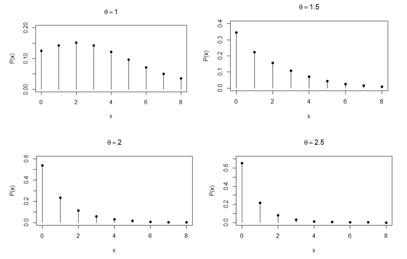
This is named as Poisson-Pranav distribution (PPD)”. The pmf of PPD presented in Figure 1.

Figure 1 Behavior of the PPD for varying values of the parameter $\theta$

Moments

The $r$ ^th factorial moment about origin of PPD (2.2) can be obtained as

${\mu }_{\left(r\right)}{}^{\prime }=E\left[E\left(X^{\left(r\right)}|\lambda \right)\right]$     ,     where $X^{\left(r\right)}=X\left(X-1\right)\left(X-2\right)\mathrm{...}\left(X-r+1\right)$       

 Using (2.1), the $r$ ^th factorial moment about origin of PPD (2.2) can be obtained as

${\mu }_{\left(r\right)}{}^{\prime }=E\left[E\left(X^{\left(r\right)}|\lambda \right)\right]=\frac{{\theta }^4}{{\theta }^4+6}{\displaystyle \underset{0}{\overset{\infty }{\int }}\left[{\displaystyle \sum _{x=0}^{\infty }{x}^{\left(r\right)}\frac{e^{-\lambda }{\lambda }^x}{x!}}\right]}\left(\theta +{\lambda }^3\right)e^{-\theta \lambda }d\lambda$   

$=\frac{{\theta }^4}{({\theta }^4+6)}{\displaystyle \underset{0}{\overset{\infty }{\int }}{\lambda }^r\left[{\displaystyle \sum _{x=r}^{\infty }\frac{e^{-\lambda }{\lambda }^{x-r}}{\left(x-r\right)!}}\right]}\left(\theta +{\lambda }^3\right)e^{-\theta \lambda }d\lambda$   

Taking $x+r$ in place of $x$ within the bracket, we get

${\mu }_{\left(r\right)}{}^{\prime }=\frac{{\theta }^4}{{\theta }^4+6}{\displaystyle \underset{0}{\overset{\infty }{\int }}{\lambda }^r\left[{\displaystyle \sum _{x=0}^{\infty }\frac{e^{-\lambda }{\lambda }^x}{x!}}\right]}\left(\theta +{\lambda }^3\right)e^{-\theta \lambda }d\lambda$   

$=\frac{{\theta }^4}{{\theta }^4+6}{\displaystyle \underset{0}{\overset{\infty }{\int }}{\lambda }^r}\left(\theta +{\lambda }^3\right)e^{-\theta \lambda }d\lambda$   

After simplification, the $r$ ^th factorial moment about origin of PPD can be expressed as

${\mu }_{\left(r\right)}{}^{\prime }=\frac{r!\left[{\theta }^4+\left(r+1\right)\left(r+2\right)(r+3)\right]}{{\theta }^r\left({\theta }^4+6\right)};r=1,2,3,\mathrm{....}$   (3.1)

Substituting $r=1,2,3,\text{and}4$ in (3.1), the first four factorial moments about origin can be obtained and using the relationship between factorial moments about origin and moments about origin, the first four moment about origin of PPD are obtained as

${\mu }_1{}^{\prime }=\frac{{\theta }^4+24}{\theta \left({\theta }^4+6\right)}$   

${\mu }_2{}^{\prime }=\frac{{\theta }^5+2{\theta }^4+24\theta +120}{{\theta }^2\left({\theta }^4+6\right)}$   

${\mu }_3{}^{\prime }=\frac{{\theta }^6+6{\theta }^6+6{\theta }^4+24{\theta }^2+360\theta +720}{{\theta }^3\left({\theta }^4+6\right)}$   

${\mu }_4{}^{\prime }=\frac{{\theta }^7+14{\theta }^6+36{\theta }^5+24{\theta }^4+24{\theta }^3+840{\theta }^2+4320\theta +5040}{{\theta }^4\left({\theta }^4+6\right)}$   

The relationship between moments about mean and the moments about origin of PPD gives the moments about mean as

${\mu }_2={\sigma }^2=\frac{{\theta }^9+{\theta }^8+30{\theta }^5+84{\theta }^4+144\theta +144}{{\theta }^2{\left({\theta }^4+6\right)}^2}$   

${\mu }_3=\frac{\left(\begin{array}{l}{\theta }^{14}+3{\theta }^{13}+2{\theta }^{12}+36{\theta }^{10}+270{\theta }^9+396{\theta }^8+324{\theta }^6+1944{\theta }^5\\ +648{\theta }^4+864{\theta }^2+2592\theta +1728\end{array}\right)}{{\theta }^3{\left({\theta }^4+6\right)}^3}$   

${\mu }_4=\frac{\left(\begin{array}{l}{\theta }^{19}+10{\theta }^{18}+18{\theta }^{17}+9{\theta }^{16}+42{\theta }^{15}+852{\theta }^{14}+3132{\theta }^{13}+2808{\theta }^{12}\\ +540{\theta }^{11}+11880{\theta }^{10}+34992{\theta }^9+20736{\theta }^8+2808{\theta }^7+59184{\theta }^6\\ +132192{\theta }^5+93312{\theta }^4+5184{\theta }^3+98496{\theta }^2+186624\theta +93312\end{array}\right)}{{\theta }^4{\left({\theta }^4+6\right)}^4}$   

The coefficient of variation $\left(C.V\right)$ , coefficient of Skewness $\left(\sqrt{{\beta }_1}\right)$ , coefficient of Kurtosis $\left({\beta }_2\right)$ , and index of dispersion $\left(\gamma \right)$  of the PPD can be obtained using following formula:

$C.V=\frac{\sigma }{{{\mu }^{\prime }}_1}$  ,$\sqrt{{\beta }_1}=\frac{{\mu }_3}{{\mu }_2{}^{3/2}}$  

${\beta }_2=\frac{{\mu }_4}{{\mu }_2{}^2}$   $\gamma =\frac{{\sigma }^2}{{{\mu }^{\prime }}_1}$ .

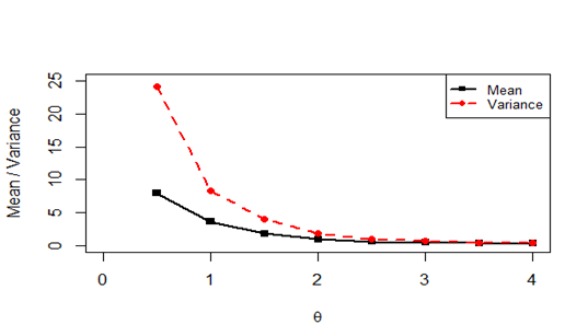
The behavior of the mean and the variance of PPD have been shown in Figure 2. Clearly PPD is always over-dispersed (variance greater than the mean).

Figure 2 Plots of mean and variance for varying values of $\theta$

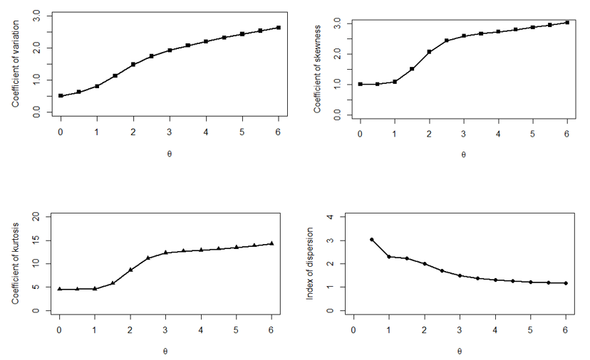
The behavior of $\text{C}\text{.V},\sqrt{{\beta }_1},{\beta }_2\text{and}\gamma$  of the PPD has been shown graphically for different values of parameter $\theta$  in Figure 3.

Figure 3 Behavior of coefficient of variation, coefficient of skewness, coefficient of kurtosis and Index of dispersion of PPD for different values of the parameter $\theta$

Increasing hazard rate and unimodality

The PPD (2.2) has an increasing hazard rate (IHR) and thus unimodal. Clearly

$\frac{P\left(x+1;\theta \right)}{P\left(x;\theta \right)}=\frac{1}{\theta +1}\left[1+\frac{2x^2+13x+17}{x^3+6x^2+11x+\theta {\left(\theta +1\right)}^3+6}\right]$  

 is a decreasing function in $x$ . Thus $P\left(x;\theta \right)$ is log-concave which means that the PPD has an increasing hazard rate (IHR) and unimodal. A detailed discussion about interrelationship between log-concavity, unimodality and IHR for discrete distributions are available in Grandell.¹³

Method of moment estimate (MOME)

Equating the population mean to the sample mean based on random sample $\left(x_1,x_2,\mathrm{...},x_n\right)$ the MOME $\tilde{\theta }$ of the parameter $\tilde{\theta }$ of PPD is the solution of the following fifth degree polynomial equation

$\overline{x}{\theta }^5-{\theta }^4+6\overline{x}\theta -24=0$ ,

where $\overline{x}$ is the sample mean.

Maximum Likelihood Estimate (MLE)

Let $\left(x_1,x_2,\mathrm{...},x_n\right)$ be a random sample of size $n$ from the PPD and let $f_x$ be the corresponding observed frequency The likelihood function $L$  and the log-likelihood function of the PPD is given by

$L={\left(\frac{{\theta }^4}{{\theta }^4+6}\right)}^n\frac{1}{{\left(\theta +1\right)}^{{\displaystyle \sum _{x=1}^k\left(x+4\right)f_x}}}{\displaystyle \prod _{x=1}^k{\left[x^3+6x^2+11x+\theta {\left(\theta +1\right)}^3+6\right]}^{f_x}}$  .

$\log L=n\log \left(\frac{{\theta }^4}{{\theta }^4+6}\right)-{\displaystyle \sum _{x=1}^k\left(x+4\right)}{f}_x\log \left(\theta +1\right)+{\displaystyle \sum _{x=1}^k{f}_x\log \left[x^3+6x^2+11x+\theta {\left(\theta +1\right)}^3+6\right]}$ .

The first derivative of the log likelihood function is given by

$\frac{d\log L}{d\theta }=\frac{12n}{\theta \left({\theta }^4+6\right)}-\frac{n\left(\overline{x}+4\right)}{\theta +1}+{\displaystyle \sum _{x=1}^k\frac{\left(4{\theta }^3+9{\theta }^2+6\theta +1\right)f_x}{\left[x^3+6x^2+11x+\theta {\left(\theta +1\right)}^3+6\right]}}$ .

The maximum likelihood estimate (MLE), $\widehat{\theta }$  of the parameter $\theta$  of PPD is the solution of the following log likelihood equation

$\frac{d\log L}{d\theta }=\frac{12n}{\theta \left({\theta }^4+6\right)}-\frac{n\left(\overline{x}+4\right)}{\theta +1}+{\displaystyle \sum _{x=1}^k\frac{\left(4{\theta }^3+9{\theta }^2+6\theta +1\right)f_x}{\left[x^3+6x^2+11x+\theta {\left(\theta +1\right)}^3+6\right]}}=0$  

This non-linear equation can be expressed in closed form and hence can be solved iteratively using Newton- Raphson method available in R-software. The MOME can be taken as the initial value of the parameter for Newton-Raphson method.

For a simulation study, we generate N=10,000 pseudo-random sample of sizes n=50, 100, 150, and 200 of a variable X having PPD). Then using Monte Carlo simulation we estimate the average bias and the mean squared error (MSE) of the MLEs of the parameter for $\theta$  =1.5, 2, 2.5 and 3.0. The formulas for finding bias and MSE of the parameter $\theta$  are

$B(\stackrel{⌢}{\theta })=\frac{1}{N}{\displaystyle \sum _{j=1}^N({\stackrel{⌢}{\theta }}_j}-\theta ),MSE(\stackrel{⌢}{\theta })=\frac{1}{N}{\displaystyle \sum _{j=1}^N({\stackrel{⌢}{\theta }}_j}-\theta {)}^2$ ).

Using following algorithm, we generate a pseudo-random sample from PPD

Algorithm

$\begin{array}{l}\text{Generate},u\sim U(0,1)\\ x\to 0\\ p_x\Rightarrow \frac{{\theta }^4\left(\theta {(\theta +1)}^3+6\right)}{{(\theta +1)}^4({\theta }^4+6)}\\ \text{while}(p_x<u)\text{do}\\ x\to x+1\\ p_{x1}=p_x*p_{x-1}\\ p_x\Rightarrow p_x+p_{x1}\\ \text{while}\\ \text{return}(x)\end{array}$

The ML estimate, biases and the mean squares error (MSE) of the parameter based on simulated data are presented in Table 3.

This table shows that bias and mean square error tends to zero for increasing sample size and increasing values of parameter. Further, MLE of $\theta$  has a negative bias in some cases.

In this section two examples of observed count datasets have been considered for goodness of fit of over-dispersed distributions namely PPD, PLD, PAD and PID. The dataset in Table 4 has been taken from Kemp & kemp¹⁴ and dataset in Table 5 has been taken from Loeschke & Kohler¹⁵ and Janardan & Schaeffer.¹⁶ The fitted plots of the distributions for dataset in Tables 4 & 5 have been presented in Figures 4 & 5, respectively.

Figure 4 Fitted probability plot of distributions for datasets in table 4

Figure 5 Fitted probability plot of distributions for datasets in table 5

A Poisson mixture of Pranav distribution named Poisson-Pranav distribution (PPD) has been proposed. Its factorial moments, raw moments and central moments have been derived. The statistical constants including coefficients of variation, skewness, kurtosis and Index of have been studied. Method of moment and maximum likelihood has been explained. Goodness of fit of PPD over Poisson distribution (PD), PLD, PAD and PID has been discussed with two examples of observed real datasets. PPD gives much closure fit over the considered distributions.

None.

The authors declared no conflicts of interest.

1. Shukla KK. Pranav distribution and its properties and applications, Biometrics and Biostatistics International Journal. 2018;7(3):244–254.
2. Lindley DV. Fiducial distributions and Bayes theorem, Journal of the Royal Statistical Society. 1958;20(1):102–107.
3. Shanker R. Akash distribution and Its Applications. International Journal of Probability and Statistics. 2015;4(3):65–75.
4. Shanker R, Shukla KK. Ishita distribution and its Applications Biometrics and Biostatistics International Journal. 2017;5(2):1–9.
5. Ghitany ME, Atieh B, Nadarajah S. Lindley distribution and its Application. Mathematics and Computers in Simulation. 2008;78(4):493–506.
6. Shanker R, Hagos F, Sujatha S. On Modeling of Lifetimes data using Exponential and Lindley distributions. Biom Biostat Int J. 2015;2(5):140–147.
7. Shanker R, Hagos F, Sujatha S. On modeling of lifetime data using one parameter akash, lindley and exponential distributions. Biom Biostat Int J. 2016;3(2):1–10.
8. Sankaran, M. The discrete Poisson-Lindley distribution. Biometrics. 1970;26(1):145–149.
9. Shanker R. The discrete Poisson Akash distribution. International Journal of Probability and Statistics. 2017;6(1):1–10.
10. Shukla KK. Shanker R. A Discrete Poisson Ishita distribution and its Application. International Journal of Statistics and Economics. 2019;19(2).
11. Ghitany ME, Al-Mutairi DK. Estimation method for the discrete Poisson-Lindley distribution. Journal of Statistical Computation and Simulation. 2009;79(1):1–9.
12. Shanker R, Hagos F. On Poisson-Lindley distribution and its Applications to Biological Sciences, Biometrics & Biostatistics International Journal. 2015;2(4):1–5.
13. Vladimir Kalashnikov. Grandell J: Mixed Poisson Processes. Chapman& Hall, London, 1997. Astin Bulletin. 2001;31(1):254.
14. Kemp CD, Kemp AW. Some properties of the Hermite distribution. Biometrika. 1965;52(3):381–394.
15. Loeschke V, Kohler W. Deterministic and Stochastic models of the negative binomial distribution and the analysis of chromosomal aberrations in human leukocytes. Biometrische Zeitschrift. 1976;18(6):427–451.
16. Janardan KG, Schaeffer DJ. Models for the analysis of chromosomal aberrations in human leukocytes, Biometrical Journal. 1977;19(8):599–612.