In this section, we defined and discuss some properties of the WLnD distribution.
The Quantile function
This function is derived by inverting the cdf of any given continuous probability distribution. It is used for obtaining some moments like skewness and kurtosis as well as the median and for generation of random variables from the distribution in question. Hyndman et al.,21 defined the quantile function for any distribution in the form Q(u) =
(u) where Q(u) is the quantile function of F(x) for 0 < u <1
Taking F(x) to be the cdf of the Weibull-Lindley distribution and inverting it as above will give us the Quantile function as follows:
(2.2.1)
Simplifying equation (2.2.1) above, we obtain:
(2.2.2)
By using (2.2.2) above, the median of X from the WLnD is simply obtained by setting u=0.5 while random numbers can be generated from WLnD by setting
, where u is a uniform variate on the unit interval (0,1) and
represents the negative branch of the Lambert function.
Skewness and kurtosis
The quantile based measures of skewness and kurtosis will employed due to non-existence of the classical measures in some cases. The Bowley’s measure of skewness based on quartiles by Kenney et al.,32 is given as;
<
(2.2.3)
while the Risti et al.,9 kurtosis based on octiles is given by;
(2.2.4)
where Q(.) is any quartile or octile of interest.
Moments
Moments of a random variable are very important in distribution theory because they are used to study some of the most important features and characteristics of a random variable such as mean, variance, skewness and kurtosis.
Let X denote a continuous random variable, the nth moment of X is given by;
(2.2.5)
Considering f(x) to be the pdf of the Weibull-Lindley distribution as given in equation (2.1.4)
Recall that from equation (2.1.4),
(2.2.6)
Let
Then, using a power series expansion for A, we can write A as:
Substituting for the expansion above in equation (2.2.6), we have;
(JKJK) (2.2.7)
Also, let
Now, considering the following formula from Tahir et al.,1 which holds for B for i≥1, and then we can write B as follows:
(2.2.8)
Where for (for j≥0) Pj,0=1 and (for k=1,2,…..)
(2.2.9)
Combining equation (2.2.8) and (2.2.9) and inserting the above power series in equation (2.2.7) and simplifying, we have:
(2.2.10)
Now,if l is a positive non-integer, we can expand the last term in (2.2.10) as:
(2.2.11)
Therefore, f(x) becomes:
(2.2.12)
Using power series expansion on the last term in equation (2.2.12), we have
(2.2.13)
Now, substituting equation (2.2.13), the power series expansion in equation (2.2.12) above, one gets:
This implies that:
(2.2.14)
Where
Hence,
(2.2.15)
Also, using integration by substitution method in equation (2.2.15); we obtain the following:
Let
;
and
Substituting for
,
and
in equation (2.2.15) and simplifying; we have:
(2.2.16)
Again recall that
and that
Thus we obtain the nth ordinary moment of X for the Weibull-Lindley distribution as follows:
(2.2.17)
The Mean
The mean of the WLnD can be obtained from the nth moment of the distribution when n=1 as follows:
(2.2.17)
The Variance
The nth central moment or moment about the mean of X, say
, can be obtained as
(2.2.18)
The variance of X for WLnD is obtained from the nth central moment when n=2, that is, the variance of X is the nth central moment of order two (n=2) and is given as follows:
(2.2.19)
(2.2.20)
The coefficients variation, skewness and kurtosis measures can also be calculated from the non-central moments using some well-known relationships.
Moment generating function
The mgf of a random variable X can be obtained by
(2.2.21)
Using power series expansion in equation (2.2.21) and simplifying the integral therefore we have;
(2.2.22)
where n and t are constants, t is a real number and
denotes the nth ordinary moment of X .
Characteristics function
The characteristics function of a random variable X is given by;
(2.2.23)
Simple algebra and power series expansion proves that
(2.2.24)
Where
and
are the moments of X for n=2n and n=2n+1 respectively and can be obtained from
in equation (2.2.17)
Some reliability functions
In this section, we present some reliability functions associated with WLnD including the survival and hazard functions.
The Survival function
The survival function describes the likelihood that a system or an individual will not fail after a given time. It tells us about the probability of success or survival of a given product or component. Mathematically, the survival function is given by:
(2.3.1)
Taking F(x) to be the cdf of the Weibull-Lindley distribution, substituting and simplifying (2.3.1) above, we get the survival function of the WLnD as:
(2.3.2)
Below is a plot of the survival function at chosen parameter values in Figure 3. The figure above revealed that the probability of survival for any random variable following a Weibull-Lindley distribution decreases as the values of the random variable increases, that is, as time goes on, probability of life decreases. This implies that the Weibull-Lindley distribution can be used to model random variables whose survival rate decreases as their age grows.
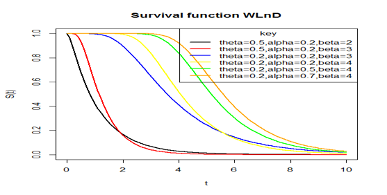
Figure 3 Plot of the survival function of the WLnD for different parameter values.
The Hazard function
Hazard function as the name implies is also called risk function, it gives us the probability that a component will fail or die for an interval of time. The hazard function is defined mathematically as;
(2.3.3)
Taking f(x) and F(x) to be the pdf and cdf of the proposed Weibull-Lindley distribution given previously, we obtain the hazard function as:
(2.3.4)
The following is a plot of the hazard function at chosen parameter values in Figure 4.
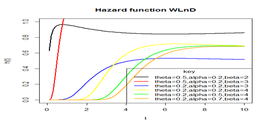
Figure 4 Plot of the hazard function of the WLnD for different parameter values.
Figure 4 above shows the behavior of hazard function of the WLnD and it means that the probability of failure for any Weibull-Lindley random variable increases as the time or age of the variable grows or increases, that is, as time goes, the probability of failure or death increases and becomes constant after some times.
Order statistics
Order statistics are used widely over the years for solving a huge set of problems such as in robust statistical estimation and detection of outliers, characterization of probability distributions and goodness of fit tests, entropy estimation, analyses of censored samples, reliability analysis, quality control and strength of materials. Suppose
is a random sample from a distribution with pdf, f(x), and let
denote the corresponding order statistic obtained from this sample. The pdf,
of the
order statistic can be defined as;
(2.4.1)
where f(x) and F(x) are the pdf and cdf of the Weibull-Lindley distribution respectively.
Using (2.1.3) and (2.1.4), the pdf of the
order statistics
, can be expressed from (2.4.1) as;
(2.4.2)
Hence, the pdf of the minimum order statistic
and maximum order statistic
of the WLnD are given by;
(2.4.3)
And
(2.4.4)
,p>respectively.
Parameter estimation via maximum likelihood
Let
> be a sample of size ‘n’ independently and identically distributed random variables from the WLnD with unknown parameters α, β and Ө defined previously. The pdf of the WLnD is given from (2.1.3) as
The likelihood function is given by;
(2.5.1)
Let the log-likelihood function,
, therefore
(2.5.2)
Differentiating
partially with respect to α, β and Ө respectively gives;
(2.5.3)
(2.5.4)
(2.5.5)
Equating equations (2.5.3), (2.5.4) and (2.5.5) to zero and solving for the solution of the non-linear system of equations will give us the maximum likelihood estimates of parameters
respectively. However, the above equations cannot be solved manually due to their complexity unless numerically with the help of statistically inclined computer programs like Python, R, SAS, etc., when data sets are available.
This section presents four datasets, their descriptive statistics, graphics and applications to some selected extensions of the Lindley distribution including the classical Lindley distribution. We have compared the performance of the Weibull-Lindley distribution (WLlD) to some families of Lindley distribution such as Lomax-Lindley distribution (LLlD), Two-parameter Lindley distribution (TPLlD), Transmuted Lindley distribution (TLlD) and the Lindley distribution (LlD).
Data sets and their nature
In this section, four different datasets and their summary are presented for fitting the above listed distributions. The available data sets I, II, III, and IV and their respective summary statistics are provided in Table 1–5 respectively as follows;
Parameters |
n |
Minimum |
|
Median |
|
Mean |
Maximum |
Variance |
Skewness |
Kurtosis |
Values |
20 |
1.1 |
1.475 |
1.7 |
2.05 |
1.9 |
4.1 |
0.4958 |
1.8625 |
7.1854 |
Table 1 Summary statistics for dataset I
Parameters |
n |
Minimum |
|
Median |
|
Mean |
Maximum |
Variance |
Skewness |
Kurtosis |
Values |
20 |
40 |
86.75 |
119 |
140.8 |
113.45 |
165 |
1280.892 |
-0.3552 |
-0.89 |
Table 2 Summary statistics for dataset II
Parameters |
n |
Minimum |
|
Median |
|
Mean |
Maximum |
Variance |
Skewness |
Kurtosis |
Data set I |
63 |
0.55 |
1.375 |
1.59 |
1.685 |
1.507 |
2.24 |
0.105 |
-0.8786 |
3.9238 |
Table 3 Summary Statistics for data set III
Parameters |
n |
Minimum |
|
Median |
|
Mean |
Maximum |
Variance |
Skewness |
Kurtosis |
Values |
59 |
4.1 |
8.45 |
10.6 |
16.85 |
13.49 |
39.2 |
64.8266 |
1.6083 |
2.256 |
Table 4 Descriptive statistics for dataset IV
Parameter estimates |
ƖƖ=(log-likelihood value) |
AIC |
A* |
W* |
K-S |
P-Value |
Ranks |
(K-S) |
0.5842 |
16.0004 |
38.0009 |
0.2483 |
0.0428 |
0.167 |
0.6324 |
1 |
1.2337 |
3.8112 |
1.1589 |
24.9726 |
53.9452 |
0.6295 |
0.1063 |
0.3113 |
0.0414 |
2 |
-0.9888 |
0.8926 |
27.2805 |
58.561 |
0.6401 |
0.108 |
0.2885 |
0.0716 |
3 |
9.7008 |
0.8162 |
30.2496 |
62.4991 |
0.6758 |
0.1141 |
0.3911 |
0.0044 |
4 |
0.361 |
29.8421 |
65.6841 |
0.6552 |
0.1107 |
0.416 |
0.002 |
5 |
9.6021 |
2.4483 |
Table 5 The statistics ll, AIC, A*, W* and K-S for the fitted models to the first dataset
Dataset I: This dataset represents the lifetime’s data relating to relief times (in minutes) of 20 patients receiving an analgesic and reported by Gross et al.,34 and has been used by Shanker et al.,35 Table 1.
Dataset II: This data represent the survival times in weeks for male rats Lawless et al.,36 (Table 2).
Data set III: This data set represents the strength of 1.5cm glass fibers initially collected by members of staff at the UK national laboratory. It has been used by Bourguignon et al.,18 Afify et al.,37 Barreto Souza et al.,38 Oguntunde et al.,39 Ieren et al.,40 as well as Smith et al.,41 Its summary is given as follows: (Table 3).
Dataset IV: This dataset represents 59 observations of the monthly actual taxes revenue in Egypt (in 1,000 million Egyptian pounds) between January 2006 and November 2010. The data has been previously used by Owoloko et al.42 The descriptive statistics for this data are as follows:
We also provide some histograms and densities for the three data sets as shown in Figure 5–8 below respectively (Table 4).
From the summary statistics of the four data sets, we found that data sets I and IV are positively skewed, while II is a bit negatively skewed or approximately normal and III is negatively skewed. Also, data sets I, III and IV have higher kurtosis while II have low level or degree of peakness.
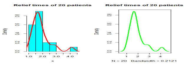
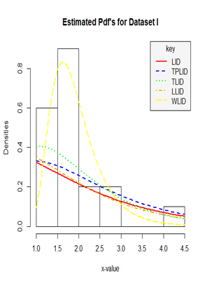
Figure 5 Histogram and density plot for the Relief times of 20 patients (Data set I).
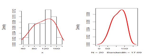
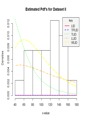
Figure 6 Histogram and density plot for the survival times in weeks for male rats (Data set II).
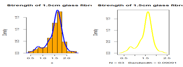
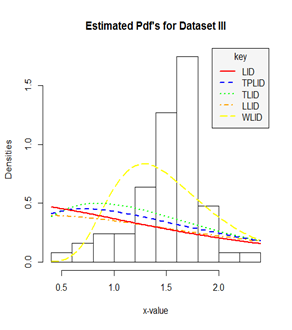
Figure 7 A histogram and density plot for the strength of 1.5cm glass fibres (Data set III).
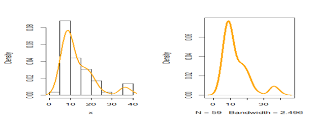
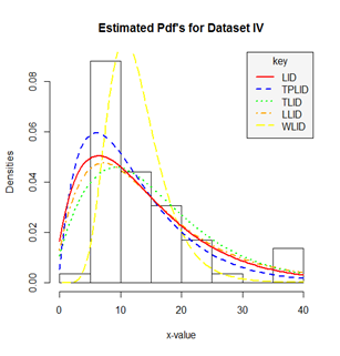
Figure 8 A histogram and density plot for the monthly actual taxes revenue in Egypt (Data set IV).
Analysis of data
These four different datasets presented above were used to fit all the above listed Lindley distributions by applying the formulas of the test statistics in section 2 in order to get the best fitted model and the results are presented as follow in the four tables for each dataset below: (Table 5).
From Table 5, the values of the parameter MLEs and the corresponding values of ƖƖ, AIC, A*, W* and K-S for each model show that the Weibull-Lindley distribution (WLlD) has better performance compared to the other four models namely: Lomax-Lindley distribution (LLlD), Two-parameter Lindley distribution (TPLlD), Transmuted Lindley distribution (TLlD) and the Lindley distribution (LlD) and hence becomes the best fitted distribution based the data set I (Table 6).
Parameter estimates |
ƖƖ=(log-likelihood value) |
AIC |
A* |
W* |
K-S |
P-Value |
Ranks |
(K-S) |
0.0278 |
106.6467 |
219.2935 |
0.4311 |
0.062 |
0.3225 |
0.0313 |
1 |
1.6862 |
1.0152 |
0.0198 |
112.8891 |
231.7781 |
0.5199 |
0.076 |
0.3772 |
0.0068 |
2 |
1.9445 |
2.8037 |
0.0371 |
128.3464 |
260.6929 |
0.4103 |
0.0586 |
0.6941 |
8.57E-09 |
3 |
0.3054 |
1.9987 |
4442.078 |
8888.156 |
NaN |
NaN |
1 |
<2.2e-16 |
5 |
0.6326 |
2.2161 |
4926.226 |
9854.452 |
NaN |
NaN |
1 |
<2.2e-16 |
4 |
Table 6 The statistics ll, AIC, A*, W* and K-S for the fitted models to the second dataset
Again the results in Table 6 above shows that the Weibull-Lindley distribution (WLlD) fits the second dataset better than the other four models (LLlD, TPLlD, TLlD and LlD) because the values of the statistics; AIC, A*, W* and K-S are smaller for the WLlD than the other models and therefore it is considered as the best fitted distribution based the data set II (Table 7).
Distributions |
Parameter estimates |
ƖƖ=(log-likelihood value) |
AIC |
A* |
W* |
K-S |
P-Value |
Ranks |
(K-S) |
|
1.4523 |
34.1708 |
74.3416 |
4.2254 |
0.7768 |
0.224 |
0.0033 |
1 |
7.6251 |
1.7248 |
|
0.361 |
81.4714 |
168.9428 |
3.074 |
0.5619 |
0.3213 |
3.60E-06 |
2 |
9.6021 |
2.4483 |
|
1.391 |
63.8482 |
131.6963 |
3.1901 |
0.5833 |
0.3413 |
6.70E-07 |
3 |
-0.9937 |
|
1.2155 |
71.0355 |
146.071 |
3.1414 |
0.5744 |
0.3427 |
5.90E-07 |
4 |
9.2573 |
|
0.9957 |
82.5853 |
167.1706 |
3.0788 |
0.563 |
0.3885 |
8.20E-09 |
5 |
Table 7 The statistics ll, AIC, A*, W* and K-S for the fitted models to the third dataset
The results from Table 7 also agrees with the previous results that the WLlD is more flexible compared to the three other models this also agrees with the fact that generalizing any continuous distribution provides a compound distribution with at least better fit than the classical distribution (i.e Lindley) irrespective of the nature of the data used provide it is asymmetry Table 8.
Distributions |
Parameter estimates |
ƖƖ=(log-likelihood value) |
AIC |
A* |
W* |
K-S |
P-Value |
Ranks |
(K-S) |
|
0.3767 |
199.8163 |
405.6327 |
0.7927 |
0.1329 |
0.1597 |
0.0986 |
1 |
8.5414 |
0.8256 |
|
0.0809 |
201.0534 |
408.1067 |
1.127 |
0.1849 |
0.1558 |
0.1139 |
2 |
6.6768 |
3.1649 |
|
0.1429 |
199.6626 |
403.3251 |
1.4251 |
0.229 |
0.1676 |
0.0728 |
5 |
-0.4154 |
|
0.1618 |
199.324 |
402.648 |
1.2489 |
0.2007 |
0.2084 |
0.0119 |
3 |
4.938 |
|
|
0.1361 |
200.6599 |
403.3198 |
1.2999 |
0.2087 |
0.1844 |
0.0361 |
4 |
Table 8 The statistics ll, AIC, A*, W* and K-S for the fitted models to the fourth dataset
Lastly, our results in Table 8 provides the same results as obtained in the above previous tables with the Weibull-Lindley distribution performing better than the other three distributions considered in this study.
The following figures displayed the histogram and estimated densities of the fitted models for the four real life data sets used in this study.
From the estimated density plots in Figures 9 we can observe that though there is no big difference between the performance of the other four models, it is very clear that the performance of the Weibull-Lindley distribution (WLlD) remains the best and consistent irrespective of the nature the datasets as compared to the Lomax-Lindley distribution (LLlD), Two-parameter Lindley distribution (TPLlD), Transmuted Lindley distribution (TLlD) and the Lindley distribution (LlD).
Furthermore, the performance of the Weibull-Lindley could be attributed to the fact that the Weibull-Lindley distribution is heavy-tailed and highly skewed to the right with excellent flexibility which allows it to take various shapes depending on the parameter values and it also exhibit some degree of kurtosis all of which are features of the four datasets used in this research, hence, the Weibull-Lindley distribution will be more appropriate for lifetime datasets which are positively skewed with a higher degree of peakness as well as those that are approximately normal with observations above zero.
Hence, having demonstrated earlier in Tables 5–8, we have a similar conclusion based on figure 3-5 that the Weibull-Lindley distribution has a better fit for the four data sets considered in this study.


