The internal flow in turbo machines is extremely complex due to the level of details of the blades, with different angles and different levels of curvature and thickness, as well as the characteristics of the channel between blades that is a direct reflection of the geometry employed, added to the phenomena caused by high speed rotation. In the literature we can find several studies that aim to improve the performance of aeronautical turbines, an arduous but necessary task, to enable the maximization of efficiency and power, thus leading to even more complex projects. Among the various possible strategies, an engineering branch specializes in computational techniques due to the agility and versatility they provide. Through a virtual prototype, it becomes possible to observe the phenomena involved and changes in contour and geometry conditions to compare the results. This study seeks the optimization of an axial turbine from a small gas turbine engine developed by ITA using Computational Fluid Dynamics (CFD) and Multi-Objective Optimization techniques focused on geometry changes to maximize the turbine performance. The simulation process will be done through the use of the commercial software ANSYS®.

Keywords: turbo-machinery, optimization, CFD, ANSYS, multi-objective, mode frontier

CAD       Computer Aided Design

CFD        Computational Fluid Dynamics

NSGA     Non-dominated Sorting Genetic Algorithm

RANS     Reynolds Averaged Navier Stokes

RMS       Root Mean Squared

SST         Shear Stress Transport

β              Blade angle

D             Characteristic Linear Dimension

ε              Turbulence dissipation rate

∅             Variable of the general transport equation

k              Kinetic turbulence energy

M            Mach number

μ              Dynamic viscosity

μ_t             Turbulent eddy viscosity

ρ              Density

Re           Reynolds number

t               Time

v              Velocity

y⁺            Dimensionless wall distance

ω             Specific turbulence dissipation rate

The aeronautical industry and its competitiveness in the market of increasingly efficient aircraft, constantly seek through a lot of research and technological development, an increasingly safe and cheap solution to the final consumer who is the passenger. These surveys can follow different goals such as: drag reduction, lift improvement, fuel economy, noise reduction, improved thermal comfort, greater ease of manufacturing, robust parts design to increase your life, increased propulsion and reduced costs generally. For each of these fields, several studies were required.

In the present work, the axial turbine used to supply power to the compressor in the propulsion system of an aircraft, known as gas turbine engine, was studied and a methodology was created for the optimization of this turbomachine in its early design phase. A suitable design of an axial turbine is aimed at generating power, efficiency and a good compromise with its performance. One of the greatest challenges is undoubtedly the adequacy and good dimensioning of its axial channel, from the inlet to the outlet of the turbomachine. Because it is a time-consuming and complex task to change and analyze the flow at each geometric change in the turbine, the use of support tools is certainly very interesting to the designer. One of these resources is the use of optimization algorithms coupled with the design tools.

A methodology has been developed to use these tools in a coupled way with the aim of providing interesting results to the designer, who can analyze different solutions for a given problem. The choice of the most appropriate design, at the end of the optimization process, is strongly dependent on what is desired for the turbomachine. The optimization technique performs searches through objective functions and constraints, adopted by the user, with the use of specific algorithms. Thus, the computational tools of the compressible and turbulent flow through the turbine were coupled with optimization models. The flow was calculated using Computational Fluid Dynamics (CFD) techniques. With the solutions of the characteristics of the flow, it is possible to determine the operational characteristics of the turbine.

Axial turbine fundamental concepts

Turbines are components that transform thermal and pressure energy into mechanical energy through the kinetic energy of the flow through the grid of the rotating system. The generated mechanical energy can be used in several ways, such as triggering another device (e.g. a compressor or a pump) or to move a generator. Essentially, the two most common types of turbines are: the radial turbine and the axial turbine. There are mechanisms to determine which type is most suitable for a particular application, for example, using the speed or specific rotation diagram. In general, for low flow values, radial turbines are more indicated. Because of the greater deflections in the flow, the radial machines transfer more energy per rotor, when compared to the axial machines. As a basic operating principle, the hot gas from the combustion chamber passing through the axial turbine is subjected to varying the amount of movement, raising the kinetic energy of the relative flow and as a consequence generating movement (rotation) of the rotor. This rotor grille then acquires mechanical power through the shaft that is absorbed by the compressor.

Computational fluid dynamics

Computational Fluid Dynamics is the area of ​​engineering that determines the general equations of fluid mechanics (continuity, momentum and energy) through approximate numerical solutions. The initial development of this technique dates back to the late 1960s, when Brian Spalding worked with his students to transform CFD from a mathematical science to a rich resource for engineers to solve real problems.¹ From established theoretical concepts, numerical and computational methods are used to calculate complex problems that would be difficult to solve by means of analytical methods. This technique uses the transport theory, heat transfer, chemical reactions and other fluid dynamics phenomena to assist the industry in the research and development of projects. CFD provides detailed and accurate flow and fluid behavior information, such as pressure, velocity and temperature distributions, forces and torques, phase distributions, flow paths, recirculation flow zones, among others.

Its application takes place in a wide range of segments, such as aerospace, automotive, biomedical, energy, chemical processes, electronic components, and can be used in all stages of the engineering process, from concept and design of new products to optimization phase, fault handling and re-design. Fundamentally, the method contains three basic steps:

1. Pre-processing: in which the CAD drawing of the proposal equipment is prepared, discretized (in computational domain) and has its boundary conditions assigned. Hypotheses and simplifications are made at this stage;
2. Processing: stage in which the computer program of high performance solves the transport equations (fluid mechanics) and other equations that model the physics and phenomena of the problem to be solved;
3. Post-processing: where phenomena involved in the case can be evaluated with the response of the calculated numerical model. At this point the user evaluates the numerical results to discuss possible design improvements and analyze the characteristics of the flow, heat transfer and mass as a whole to each engineering problem.

Governing equations

The laws of conservation respect Lavoisier's observations of more than 200 years: In a chemical reaction done in a closed vessel, the sum of the masses of the reactants is equal to the sum of the masses of the products. From his remark, the famous phrase "In nature nothing is created and nothing is lost, everything is transformed" was created. In mathematical terms we can prove this by means of a control volume, shown in Figure 1.

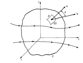
Figure 1 Space defined system.²

Through the balance in this control system and the use of the divergence theorem it is possible to arrive at the differential form of the transport equation, as in Equation 1.

$0=\frac{\partial \rho }{\partial t}+\overrightarrow{\nabla }\cdot \rho \overrightarrow{v}$ (1)

The equation can be presented in terms of mass, momentum and energy after the imbalance on the control system. After some rearrangement it is possible to express the general transport equation, present in Equation 2, or general transport equation of $\varnothing$ variable:

$\frac{\partial }{\partial t}\underset{V}{\overset{}{{\displaystyle \int }}}\rho \varnothing dV+\underset{A}{\overset{}{{\displaystyle \oint }}}\rho \varnothing v.dA=\underset{A}{\overset{}{{\displaystyle \oint }}}{\Gamma }_{\varnothing }{\nabla }_{\varnothing }\cdot dA+\underset{V}{\overset{}{{\displaystyle \int }}}{S}_{\varnothing }dV$ (2)

The structure of this equation is the basis of all CFD methods and shows a transient term followed by a convective, a diffusive and finally the source term. On this equation the continuity, momentum and energy equations can be expressed after the $\varnothing$ variable is respectively changed by the mass, velocity and temperature. For a discrete domain, each cell volume will need to have all of these expressions solved.

Turbulence

The study of turbulence remarks the time of the notable Leonardo Da Vinci, around 500 years ago. In a very clever way, he was able to understand the effects of turbulence by comparing this phenomenon to the movement of human hair.³ Nowadays it is well known that a flow can be classified in three different ways: laminar, turbulent and transitional. The Reynolds number, from Equation 3, is used to help in this classification.

$Re=\frac{\rho vD}{\mu }$ (3)

The turbulence is a characteristic of the flow and not of the fluid, and as a consequence the general characteristics of the turbulence are respected for all fluids.⁴ Due to this, the turbulence behavior can be modeled to save the trouble of calculation all the turbulent scales associated to the problem (Figure 2).

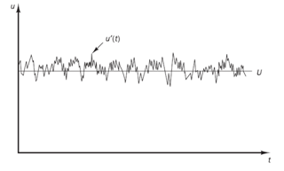
Figure 2 Velocity fluctuation.⁵

There are several turbulence models common to both research labs and industry. For this paper the chosen method is RANS, or Reynolds Averaged Navier Stokes. This methodology models all turbulent structures on the domain in order to provide good stationary resolution for most engineering applications.⁶ This project solves the compressible flow equations by the use of the SST turbulence model, which was proposed by Menter in 1993 and represents an enhanced k-ω model.⁷ Previous works have shown that this is an appropriate model for solving 3D turbulent flow simulations applied to turbomachinery.^8-11 The main reason for the success of this model is its ability to work as a k-ω model near the walls and as a k-ε model away from the walls. This behavior adds versatility to the calculation, as the model can automatically change to the most interesting methodology to capture the main manifestations in each domain region.⁵

$\frac{D\left(\rho \omega \right)}{Dt}=\nabla \left[\left(\mu +\frac{{\mu }_t}{{\sigma }_{\omega }}\right)\nabla \omega \right]+\alpha \frac{\omega }{k}{P}_k-\beta \rho {\omega }^2+\rho \frac{2\left(1-F_c\right)}{{\sigma }_{\omega }\omega }\nabla k\nabla \omega$ (4)

Optimization

The optimization process enters into the traditional design flow by suggesting that, after proof of performance of the study equipment is realized, modifications are proposed and studied in order to further improve the operation of this project. The cycle of a project is expressed below in Figure 3.

The concept stage aims to raise market needs, technological possibilities for implementation in the project and economic feasibility of the investment. After this study, planning is performed for the purpose of mapping the user to the product being developed, their technical requirements, required research, their use and operation as well as specification. Finally, in the stage of product engineering, issues such as design, design calculations, simulations and optimizations, validations and prototyping are discussed to allow this product to be made.¹² After this step, design begins, at which point the objective esthetic is defined. Then the project starts, when the necessary items are defined, sized and specified. The analysis stage begins, in which simulations will be performed to estimate the product behavior. If it is found that the operation with the current project is compromised, improvements are proposed. After this, the study optimization can be contemplated, process in which objectives and goals are established and modifications are realized in the model with the aim of improving its performance. As this process leads to modifications, new analyzes must be performed and only at the end of this cycle should the product be referred to the generation of a prototype, for validation and finally production, saving unnecessary costs with intermediate prototypes.¹³

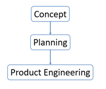
Figure 3 Cycle of general engineering projects.¹²

This cycle from Figure 4 can lead to an uncountable number of modifications, which consequently require a countless number of simulations. To avoid infinite possibilities, cases are elaborated using optimization methods. In these methods the variables to be worked are defined, that is to say, which parameters are susceptible of modifications in the model, along with the objectives of this process. At the end of these definitions one must choose an optimization method, which is nothing more than a search technique in which a finite number of cases will be studied and a curve or response surface is generated in order to estimate a possible optimal point of design, or even a point of improvement. After applying these techniques, the analysis of the points obtained for validation of the estimated data with the data obtained by simulation should be performed. This process allows the response to be obtained with a reduced number of simulations and consequently, less time (saving computational effort).

Figure 4 Product life cycle development.

Most engineering real problems cannot be expressed in single goal optimization. For multiple-objective cases it is usual that the objectives are conflicting, in order that it is not possible to determine one single optimized configuration.¹⁴ To solve this kind of problem genetic algorithms were developed around 1970.¹⁵ Genetic Algorithms start their search from a randomly created initial population. From this set of individuals, the adaptation or individual quality of each is analyzed and only a few individuals are preserved for the next generation. The decision criterion is the non-dominated or Pareto-optimal solutions, that is, solutions that cannot be improved independently of the objective unless the worsening of another objective occurs.¹⁶ With the solutions of the population, called the parents, crossing and mutation operators are applied in order to generate a new population, called a descendant, that will be closer to the final response than the previous generation. The process continues in this cycle until the stop condition is reached, as shown in the flowchart shown in Figure 5 elaborated by Deb et al.¹⁷

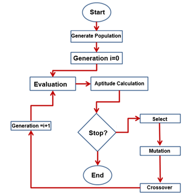
Figure 5 Flowchart of genetic algorithms.¹⁷

The NSGA method, proposed by Professor Deb and his colleagues¹⁷ is a method of regular accuracy and low convergence rate.¹⁸ However, it is fast and robust, being able to operate continuous and discrete variables and creating new populations in regions statistically more interesting for the calculation.¹⁹ Another advantage of this algorithm is its ability to allow different scenarios to be studied in parallel. For computers with adequate configuration this feature can be a differential to get the problem response in reduced time. This algorithm was developed to overcome the main criticisms of the models that existed until then, including the NSGA model, which presents high computational cost, the need for an operator, called a sharing parameter, that raises the level of difficulty of using the technology, and the lack of elitist reproduction, which shows itself as a great performance accelerator of genetic algorithms.¹⁷

This model discards the need to use the sharing operator when using a population comparison approach, thus eliminating the need for user intervention to define this parameter. In addition, Deb and his colleagues have demonstrated several cases in which the benefits of using this algorithm are clear. While the NSGA model compares each individual to all others, the improved model analyzes the individual and separates them into a selected group, and the next solution will be compared to this particular group. With this, the concept of elitism is used, in which the algorithm establishes relations to determine the best individuals for the calculation of the next generations. Because of this feature, its convergence rate is high quality, although slow.

In Figure 6, an outline of the proceedings of the NSGA-II algorithm is shown. The main operation starts with a population $P_0$ . For each solution obtained, a ranking is assigned in ascending order, in which level 1 is the best, followed by level 2 and so on. After the mutation and crossing operations, the population $Q_0$ is obtained. From the combined population of $P_0$ and $Q_0$ , solutions F are obtained from the distances D of each solution for the objectives. Those individuals who present the longest distance are rejected while those of the shortest distance are preserved for the next generation. This process is given by the Equation 5:

$D=F_{i+1}-F_{i-1}$ (5)

The elitism concept used in the NSGA-II algorithm is responsible for the disposal of less able individuals on behalf of the population that shows itself more adapted to survive until the next generation, in which it will be combined with other elements giving rise to a new elitist process. Through these operations it becomes possible to select the most suitable individuals for the objectives contemplated. Finally, in addition to all the qualities presented above, this model was chosen for the current research because of its great expression in the most recent works of optimization of turbomachinery, showing the current trend of the application of optimization algorithms in this specific branch of knowledge. As an example, the works of Zhu et al.,²⁰ of Patrao et al.,²¹ of Torabi et al.,²² of Zhu et al.,²³ Wang et al.,²⁴  and Wang et al.,²⁵  and Amaral et al.²⁶

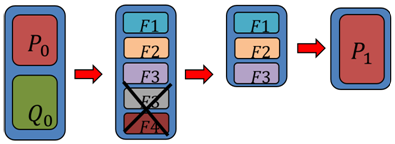
Figure 6 NSGA-II algorithm proceedings.¹⁷

The present work makes use of the project developed in previous work,²⁷ in which preliminary data of an axial turbine with generated power of 1,722 MW, adiabatic efficiency of 88.5% and the torque in the axis of 584.092 Nm for the specified gas turbine. The present project started at this stage. From the data provided as boundary conditions and the virtual prototype of the turbine (Figure 7), the model was elaborated in the computational solutions using other software for the determination of turbulent 3D flow and optimization. The steps of modifying the geometry, mesh generation, calculation and analysis of the results were performed at ANSYS tools, while the optimization tool used was Esteco’s ModeFRONTIER. We chose to use a few different tools to ensure the robustness of the process developed here and the main advantage of working with only two software suppliers was the ease of coupling these tools. The entire study model was made in ANSYS Workbench, which made it possible to generate the model setup in an automated way. Each distinct project that was proposed by ModeFRONTIER was imported by ANSYS, which in turn was able to reproduce all discretization definitions, physical problem definitions and post-processing capabilities for each situation. This robustness is of great importance because it allows a large number of different geometries to be studied in an automated way without tools conflicts of communication and without the necessity of manual scripts created by the user.

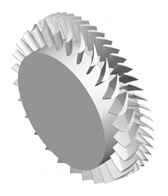
Figure 7 CAD model of the rotor and stator of the machine stage.²⁷

The use of computational tools

Initially the CAD model was edited in ANSYS SpaceClaim v18.0 software, an advanced CAD modeling tool to prepare the model for a simulation analysis in which geometric elements unnecessary for the study were eliminated. Then the design was created on Blade Modeler software, a module capable of extracting mathematically the topology of curvature of high complexity of the faces of the profile. Reference axes must be respected and the domain entry and exit must be properly delimited. The main benefit of this tool is its ability to recreate the design of the turbine with parameterizable form. This is a common procedure in turbomachinery optimization studies, since the researcher has more access to the geometric variables of the case for future optimization studies and avoids the use of multiple platforms from different suppliers, which approach may prove to be less, especially when working with optimization tools.

The generation of the fluid domain is created in this step, starting from the geometry of the blades that were properly worked and recreated with the use of parameters. The domain created is shown in Figure 8, and it is composed of the following parts: an inlet; an outlet; an interface region between the stator and rotor domains; walls representing the blades, the hub and the shroud and faces of periodicity, because the created mathematical domain considers only a stator blade and a blade of the rotor in order to save computational effort.

The parameterizable model extracted by the Blade Modeler software has another advantage: it can be easily coupled to the Turbogrid software (both of them of the ANSYS Workbench v.18.0 platform), a tool that has advanced mesh generation capabilities for turbomachinery and allows the generation of hexahedral mesh and of good quality with due refinement, especially in the regions of the leading and trailing edges of both blades. With this, the discrete mathematical model is created. The mesh generated, shown in Figure 9, is then exported to ANSYS CFX v.18.0 software, a commercial tool in the academic and industrial sector for three-dimensional calculation of computational fluid dynamics (CFD) of turbomachinery and various other engineering problems. The domain of study has an inlet, an outlet, two periodic interfaces and an interface to realize the communication of the stator domain with the rotor domain of the rotor. Further details on the mesh will be presented in subsequence paragraphs.

Figure 8 CAD model of the rotor and stator of the machine stage.²⁷

Figure 9 Discrete model of the study domain.

Mesh independence study

When modeling a given problem, it is necessary to ensure that the model represents the real case reliably. In this sense, an important analysis is the resolution of the mesh used, since the numerical methods are strongly dependent on the quality of the computational mesh. It is easily observed that the result of a simulation is remarkably sensitive to the number of elements in use. In general, the greater the number of mesh elements that discretize the domain, the greater the level of accuracy of the results obtained. However, overly refined meshes require a lot of computational power for calculation and do not necessarily provide more accuracy. Thus, a strategy is needed to analyze the independence of the results in relation to the mesh used, so that the mesh less refined and, that is able to capture the phenomena of interest, is used in the numerical studies.

In this way, it becomes necessary to study mesh convergence (and independence). A study was carried out comparing the results of a physical model variable for different mesh sizes so that it is easy to visualize the point at which we have the ideal mesh, refined enough to capture all the desired phenomena involved, but not overly refined delay the study. In this case the value of the Mach number in a region of the extrados zone of the blades and the power generated by the machine is measured. These data were chosen because the power is a relevant data and of interest for the study as a whole, while the monitoring of a point variable like Mach is ideal to better map fluctuations that occur in the domain, since parameter-weighted monitoring such as areas, flow or volumes tend to amortize this characteristic. In Table 1, the results of the mesh convergence study are presented.

Figure 10, shows the evolution of power and Mach number with the number of elements of the mesh.

Figure 10 Evolution of the results of the mesh study.

The study presented above is common for several CFD applications, however it is little used in turbomachinery design due to its inability to show in a more detailed way the evolution of the results with different meshes for different points of the domain. Because of the high complexity topology of the blades it is interesting to survey more comprehensively, monitoring other properties that are modified due to the discretization employed. Thus, the distributions of pressure, temperature, total pressure, total temperature and Mach from the blade hub to its top were also evaluated. The values ​​of y+ and its distribution on the walls of the domain should also be evaluated. The mesh independence study exhibits the point at which the mesh converged and the case was no longer dependent on the mesh refining level. Possible uncertainties regarding the level of accuracy due to discretization are eliminated by this strategy.

The mesh with about 7.7 million elements is able to represent the model used for both variables that were monitored during the process, but nevertheless presents the maximum y+ value of 4 in the walls. The value is above that recommended by the literature for the turbulence model used in the present work. However, the mesh that respects the recommended value of y+ <1 presents more than 10 million elements and did not present significant differences in the variables monitored.

As the difference in the simulation time between these two meshes is relevant and the same cannot be said in relation to the differences of the captured results, the mesh parameters of 7.7 million elements were used as reference throughout the work. The technical library of the tool informs that for values ​​of 2 < y+ > 30 in the turbulence model used (k-ω SST), the scalable wall law is applied, that is, although no significant differences in results were obtained for the meshes of 7,7 million and 10 million elements, there is a relevant difference with respect to the form that the calculation in the boundary layer is obtained. Meshes that present the value of y+ > 2 model the turbulence in the boundary layer, while meshes that respect the value of y+ < 2 effectively calculate the flow phenomena present in the boundary layer.

The mesh independence study is presented by Figure 11.

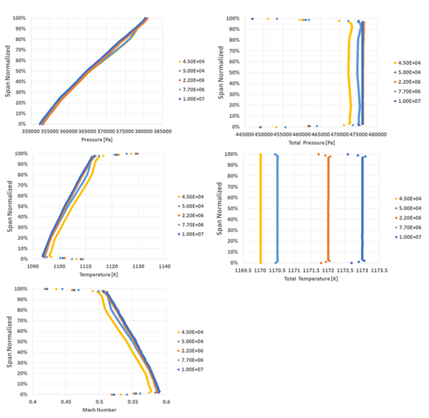
Figure 11 Comparison of the distribution of properties of interest from the base to the top of the blade at the leading edge of the stator for different meshes.

In these images, there are several points in which the results of these two meshes overlap, making possible to observe that there is no relevant variation of performance. Table 2 shows in details the level of difference between the meshes of 7,7 million cells vs. 10 million cells.

In the possession of all the above data it was decided to use the 7.7 million elements mesh as reference for the present study, since it demonstrates good reliability with the results and a shorter calculation time when compared with the most refined meshes.

Results from the original axial turbine

This study considered the response as converged from the point of view of the residuals when the results reached the level of RMS < 10E-6, which is below the standard residual values ​​that are most commonly used in this CFD software, RMS <10E-4. Also, physics stabilization and numerical balance were also evaluated to ensure convergence. The pressure contour calculated can be observed at Figure 12. The pressure distribution demonstrates the evolution of this property in the direction of the flow and allows the visualization of the high pressure zone at the entrance of the domain and the reduction of its magnitude in the downstream (stator-rotor) direction. Furthermore, it is possible to view low pressure zones after the trailing edge of the rotor blade.

Performance data comparing the CFD study with the previous theoretical values is presented through Table 3.

Figure 13 shows the good correlation between the values ​​determined in the preliminary design of the axial turbine using 1D modeling with the results of the solution of the calculation of the 3D flow using the technique of CFD. In the regions near the hub or at the shroud, a slight change of values is observed, as a result of the variation of the kinetic energy of the flow due to the existence of the boundary layer. Also, it is clear the absence of hot spots that prejudice the machine operation. There are distinctions of the results at the rotor blades, which means that there is an indicative that the design could be recalibrated.

Figure 12 Pressure contour at the flow path.

Figure 13 Comparison of variables distribution along the height of the rotor blade.

For the optimization process, different variations were considered for the blade angles, which were properly parameterized to be used by the genetic algorithm in the evolutionary process. These angles were considered at different heights for each blade. Five heights were used: the hub, the top and three more intermediate and equidistant heights of the blade. For each of the heights described above, seven values ​​of β were used to model the angles of each blade, traversing its leading edge geometry to the trailing edge. From five distinct heights, and seven parameters defined by height there are 35 input parameters for the study of a spade. Since the stage consists of a stator blade and an impeller blade, there are 70 input parameters to be evaluated.

A multiobjective optimization study, a problem with the level of complexity as described above, and the mesh quality already presented considering seventy different parameters, is not feasible to be solved. Because of this reality, different techniques were considered to simplify the proposed problem and thus to obtain data in a shorter time. It was considered the possibility of working with curvature adjustment or response surface techniques, as presented by Liu et al.,²⁸ in which a correlation between the parameters based on the original problem to be studied was created. These strategies were rejected to increase the reliability of the study here, reducing errors with oversimplifications of the mathematical model. However, due to the difficulty of carrying out such a complex study with so many input parameters, a solution already used in other studies that have encountered this same limitation has been adopted, as published by Kammerer et al.²⁹ Sensitivity analysis (Figure 14) were performed to study which angles are most relevant to the expected objectives-to increase power and efficiency, and to allow the optimization process to disregard input parameters that cause less impact on responses in favor of other more interesting parameters.

Before the optimization process, a sensitivity study was proposed to help in understanding the relevance of all the parameters involved and to enable the most interesting ones to be chosen for the defined objectives. For the elaboration of the sensitivity analysis one must create variations of the original design and solve each one of these different simulations. With this, the optimization tool is able to correlate the changes occurring in each new project and to work with election criteria to determine which ones are most pertinent to be worked on. Using the native tool of generating projects with random variations of the original model, respecting a range of possibilities previously defined by the user, more than 1,400 different simulations were performed. This methodology and procedure allowed the understanding that the root and top angles of the stator and rotor had very low impact on the determined targets, when compared with the other parameters created at intermediate heights of both blades. Due to the low effect of these variables, the decision was made, based on the good practices of turbomachinery projects, to discard them from the optimization process. The fact that these parameters have not been chosen to remain in the optimization process does not mean that they have no impact on the results. The conclusion of this step is that there are more relevant parameters in which greater dedication is justified along the heuristic goal process.

Figure 14 Power and efficiency sensitivity charts.

The objective of the optimization study is to maximize power and efficiency in turbine operating conditions. The initial population given was achieved by random initialization, taking advantage of individuals created for the sensitivity study, so that a large spectrum could be studied. By this approach, the number of parameters could be reduced from 70 to 49. Then all the projects used for this study were used to feed the heuristic model and serve as the starting point for the optimization process using the NSGA model -II.

Results from the original axial turbine

The optimization algorithm based on genetic code has as a characteristic the evolution from generation to generation and allows the construction of the Pareto Front, which expresses the various solutions that can be used for the project. As expected, there are a large number of solutions present in the Pareto Front. A single, perfect and ideal solution is not possible for multiobjective problems since any solution obtained from Pareto Border is unable to improve one goal without harming others. There is no single possibility to be used to achieve the required objectives, but the implemented genetic algorithm has been able to find several distinct design points that are equivalent, in addition to surpassing the original design obtained by the midline theory. The genetic algorithm worked with 35 evolutionary generations until its convergence criterion was reached. The process calculated more than 8700 distinct individuals, each individual presenting a different design of this turbine. For the calculation of all these analyzes a cluster with Intel Xeon processors of 3.0 GHz and 32 nodes was used. The total simulation time was 2920 hours, which is equivalent to about 4 months of calculation.

The genetic code applied its mechanisms of evolution (crossing and mutation) until the criteria of numerical convergence was reached. Remembering that the decision to stop in the numerical solution is function of the user experience about the engineering problem being analyzed. Several individuals were determined over the 35 evolutionary generations, which were necessary for the code to reach its convergence. Figure 15 shows all the individuals that were simulated throughout the process. Its color pattern is in function of the number of generations, being dark blue the results of the first generations and red the projects obtained in the last generation of the process.

Figure 15 Individuals calculated by the genetic algorithm.

The Pareto Front obtained, expresses the several possible projects of this machine so that the proposed objectives are reached. The Pareto Frontier demonstrated by Figure 16 shows all the different projects that were obtained from modifications in the original machine, to the detriment of improving each one of the objectives of study. In the vertical axis is expressed the efficiency of the set while in the horizontal axis is the power generated. As expected, there is no single project that meets the proposed objectives and the Pareto Frontier has the function of demonstrating possible modifications that are equivalent to each other, since each project presents greater improvement for one objective to the detriment of the other.

Figure 16 Pareto front.

In order to compare different results of this Pareto Border, three different projects were chosen to analyze the results. These projects were named as: Optimized 1: the Pareto Border higher efficiency point; Optimized 2: the "global" point in which a project was tried that benefits both efficiency and power generated; Optimized 3: the highest Pareto border power point. For the decision of what these points were, a graph in Figure 17 was drawn from the Pareto Frontier with the purpose of dimensioning the obtained data and facilitating the visualization of the proposed projects for analysis of results.

For these three different projects, the distribution of the properties and the characteristics of the flow were evaluated, in a similar way to what was already demonstrated in the mesh convergence study. For the leading and trailing edges of the stator and rotor blades, the relative Mach number distributions, static pressure, relative total pressure, static temperature and relative total temperature were raised, as can be observed at Figure 18.

Figure 17 Gain of the Pareto Frontier.

Table 4 presents the comparison between the original turbine design and the three optimized designs, which were selected for post-processing.

It is noticed that, as indicated by the Pareto Frontier, the answers obtained are equivalent to each other, but they may privilege one objective over another, which is common in the design of these machines, since there is a distinction between what is a high performance and what is a high efficiency. Thus, it is observed that the optimized design 1 presents values ​​of efficiency much higher than the original one, with an increase of about 1.5% in the measured efficiency, while the generated power was impaired and presented lower values ​​than the original machine. The optimized design 3, in turn, presents higher values ​​of generated power (7.7% higher), but its efficiency was also impaired when compared to the original machine. This characteristic was expected, since the output parameters (Power and Efficiency) are conflicting with each other. For this reason, it is proposed the optimization analysis by genetic algorithm to investigate different projects that could benefit both objectives.

The design Optimized 2 is in the range of possibilities of the Pareto Frontier that surpass the performance of the original project for both objectives, with an increase of 0.8% in efficiency and more than a 3% increase in the power generated. Among the possibilities selected here, this project was more interesting because it privileged both objectives and was selected to be compared in other post processing with the original design. The blade-to-blade view is an interesting resource for flow analysis along the domain of turbocharged engines. In an analogous way to that used to present the partial results, it was opted for the analysis of the results in the solution 2. When analyzing the pressure gradients in a comparative of the original model in relation to the model obtained through the genetic algorithm it becomes clear the greater smoothing and homogenization of the disturbance. The reduction of the shocks found in the rotor blades is also clear, through Figure 19.

In general, part of the flow presents the same aspect as that observed in the original model, as region of greater velocity in the dorsal of the blade, zones of stagnation and mat characteristic of the profile. However, the contours above present smoother results, making the flow more efficient. From isosurfaces, the region in which the presence of zones with M> 1 occurs is clear and how that region was attenuated at the end of the optimization process. In the region close to the rotor there are small areas of Mach> 1 and it is clear that this was the region of greatest benefit of this characteristic through the genetic code. The improvement that is observed in the performance of this equipment is the result of this reduction of shock zones, which impose losses on the system, as shown in Figure 20.

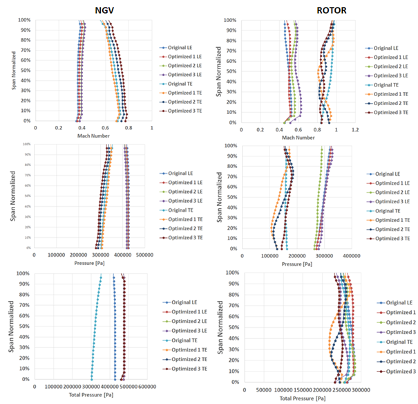
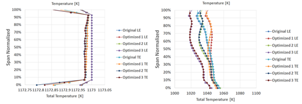
Figure 18 Distribution of absolute properties: Mach number, Pressure, Total Pressure, Temperature and Total Temperature for both NGV and Rotor.

Figure 19 Comparison of the static pressure gradient in the original model vs optimized for the blade height of 50%.

Figure 20 Isosurfaces of value M = 1.

In order to understand the modifications between these two projects, an overlap of both geometries-Original and Optimized 2-is presented in Figure 21, with the original blades being in the translucent gray color and the optimized in the opaque blue color. It is observed that the geometry presented here was obtained under a single analysis of the effects of computational fluid dynamics, and the performance improvement was due to the reduction of the bubble zone, or clogging, that occurs in the machine in regions of high Mach values. No manufacturing limitations, as internal cooling of the blades, materials and alloys, were considered at the present study nor analyzes of structural fatigue and thermal fatigue.

Figure 21 Comparison of original and optimized 2 blade geometries.

The results of the original machine analysis enabled the identification of the property distributions along the domain of study. It was observed the evolution of the static pressure and total pressure in the axial direction of the flow, with reduction in the downstream direction as expected. It was also identified the presence of shock waves, a common phenomenon in axial turbines due to the high velocity values ​​involved. There was little variation in the thermal load as the flow flows between the channels of the stator blades to the channels of the rotor blades, which follows with as it was expected since this energy is not used for the work generation. A sensitivity study was carried out to determine the relevance of the various parameters that were created from the original angles of the stator and rotor blades for the modifications of the expected responses to the study: the improvement of the power and efficiency of this stage. The sensitivity study developed allowed to understand which parameters are the most relevant to achieve these objectives, and the impact of the intermediate section angles of the blades was clear when compared to the angles present at the root and at the top. This methodology allowed to reduce the number of input parameters of this problem from 70 to 49, whose benefit was explored in the elitist heuristic process performed in the sequence. One of the projects obtained was chosen for study - the project titled Optimized 2. This project presented a 0.8% increase in efficiency and more than 3% in the power generated.

The results obtained from this methodology provided the obtainment of projects optimized in relation to the original machine and verified that the use of methodologies based on genetic algorithm is effective to improve turbomachinery projects. The methodology presented here was able to couple CFD and multiobjective optimization techniques with genetic algorithm effectively and provided adequate results for the improvement of the original machine. With the Pareto frontier obtained, it is up to the designer to define which distinct design will be used based on the various possibilities obtained, in which one output parameter is the most benefited when compared to the other. In this way, the choice will be dependent on the engineering decision to work with a more efficient or more powerful machine. The proposed methodology can be reproduced in other stages of the same turbine and even in other projects, whether turbomachinery or not. The association of CFD techniques with genetic algorithm demonstrates a viable path for obtaining better engineering projects. The technology is recent, if studied in a timeline of engineering techniques, but its effectiveness and gains ensure ample space to be even more used in various industry sectors.

Multiobjective optimization studies are increasingly present in several sectors of the industry and are present in the most recent researches of fluid dynamics improvement of turbomachinery. This technology makes it possible to obtain relevant data in a timely manner. The process of developing a new axial turbine takes time and optimization algorithms proposes to increase productivity and even to obtain non-intuitive designs in attractive time, especially in the highly competitive scenario of this industry. As a suggestion for future studies, a natural evolution for this study would be a new optimization process from the consideration of all input parameters. The sensitivity study proposed here aimed at reducing the total number of parameters that would be used in the analysis to accelerate the results, so that new studies could contemplate all these parameters to verify if this decision would lead to modifications in the Pareto Frontier and until even if there is the possibility of a new Pareto Frontier technically superior to the one found here. Also, fluid structure interaction simulations could also be performed to study heat exchange, flutter and other pertinent phenomena.

None.

Authors declare that there is no conflict of interest.

1. Runchal AK. Brian Spalding: CFD & REALITY. ICHMT International Symposium on Advances in Computational Heat Transfer; 2008.
2. Anderson J. Computational Fluid Dynamics. 1st ed. McGraw-Hill Education; 1995.
3. Ecke ER. Turbulence Problem: An Experimentalist's Perspective. Los Alamos Science. 2005;29:124‒141.
4. White FM. Fluid Dynamics. 6th ed. McGraw-Hill; 2007.
5. Versteeg HK, Malalasekera W. An Introduction to Computational Fluid Dynamics. 2nd ed. Harlow: Pearson Education Ltd; 2007.
6. Wilcox DC. Turbulence Modeling for CFD. DCW Industries Inc.; 1993.
7. Menter FR. Two-Equation Eddy-Viscosity Turbulence Models for Engineering Applications. AIAA Journal. 1994;32:1598‒1605.
8. Bardina JE, Huang PG, Coakley TJ. Turbulence Modeling Validation Testing and Development. NASA Technical Memorandum; 1997. 100 p.
9. Bardina JE, Huang PG, Coakley TJ. Turbulence Modeling Validation. AIAA paper; 2012. 97‒121 p.
10. Simões MR, Montojos BG, Moura NR, et al. Validation of turbulence models for simulation of axial flow compressor. 20th International Congress of Mechanical Engineering; 2009. 9 p.
11. Tomita JT, Silva LM, Silva DT. Comparison between Unstructured and Structured Meshes With Different Turbulence Models for a High Pressure Turbine Application. ASME Turbo Expo: Copenhagen, Denmark; 2012.
12. Rozenfeld H, Forcelllini FA, Amaral DC, et al. Product Development Management-A Process Improvement Reference. Editora Saraiva; 2006.
13. ANSYS Inc, CFD Training material; 2016.
14. Konak A, Coit DW, Smith AE. Multi-objective optimization using genetic algorithms: A tutorial. Realiability Engineering and System Safety. 2006;91(9):992‒1007.
15. Holland JH. Adaptation in natural and artificial systems. Ann Arbor: University of Michigan Press; 1975.
16. Pérez MAF. A heuristic method for the multiobjective scale problem in various machine environments. Masters Dissertation; 2012.
17. Deb K, Pratap A, Agarwal S, et al. A Fast and Elist Multiobjective Genetic Algorithm: NSGA-II. IEEE Transactions on Evolutionary Computation. 2002;6(2):182‒197.
18. Jones DF, Mirrazavi SK, Tamiz M. Multi-Objective Meta-Heuristics: An Overview of the Current State-of-The-Art. European Journal of Operational Research. 2002;137(1):1‒9.
19. ModeFrontier user Manual. Esteco webinar series; 2016. 39 p.
20. Zhu J, Cai X, Gu R. Multi-Objective Aerodynamic and Structural Optimization of Horizontal-Axis Wind Turbine Blades. Energies; 2017.
21. Patrao AC, Villar GM, Tomita JT, et al. An optimization plataform for high speed propellers. Aerospace Technology Congress: Solna, Stockholm; 2016. 17 p.
22. Torabi SHR, Alibabaei S, Bonab BB, et al. Design and Optimization of turbine blade preform forging using RSM and NSGAII. Journal of Intelligent Manufactoring. 2017;28(6):1409‒1419.
23. Zhu GJ, Guo PC, Luo XQ, et al. Wind turbine blade geometry design based on multi-objective optimization using metaheuristics. 26th IAHR Symposium on Hydraulic Machinery Manufactoring; 2012.
24. Wang L, Wang TG, Luo Y. Improved non-dominated sorting genetic algorithm NSGA-II in multi-objective optimization studies of wind turbine blades. Applied Mathematics and Mechanics. 2011;32(6):739‒748.
25. Wang X, Hirsch C, Kang Sh, et al. Multi-objective optimization of turbomachinery using improved NSGA-II and approximation model. Comput Methods Appl Eng. 2011;200(9-12):883‒895.
26. Amaral LGF, Tomita JT, Bringhenti C, et al. Optimization of an Axial Turbine Used in Small Gas Turbine Engine Based on 3D Simulations. ISABE - International Society for Air Breathing Engines; 2017.
27. Martins VAC. Preliminary Design of an Axial Turbine for Use in Small Power Gas Turbine. São José dos Campos: São Paulo, Brazil; 2011.
28. Liu Y, Manesso E, Gunawan R. Reduced dimension ensemble modeling and parameter estimation. Bioinformatics. 2005;31(20):3387–3389.
29. Kammerer S, Mayer JF, Paffrath M, et al. Three-dimensional optimization of TurboMachinery Blading Using Sensitivity Analysis. ASME Paper; 2003.
30. Croba D, Kueny J. Numerical Calculation of 2D Unsteady Flow in centrifugal Pumps: Impeller and Volute Interaction. International Journal for numerical Methods in Fluids. 1996;22(6):467‒481.
31. Aberdeen Group; 2015.
32. Procedure for Estimation and Reporting of Uncertainty Due to Discretization in CFD Applications. Journal of Fluids Engineering. 2008;130(7):078001.
33. Oberkampf WL, Trucano TG. Verification and Validation in Computational Fluid Dynamics. Progress in Aerospace Sciences. 2002;38(3):209‒272.
34. Japikse D. Turbomachinery Performance Modeling. SAE Technical Paper; 2009.
35. Saravanamuttoo HIH, Rogers GFC, Cohen H. Gas Turbine Theory. 5th ed. Prentice Hall; 2001. 510 p.
36. Baskharone EA. Principles of Turbomachinery in Air-B reathing Engines. Cambridge University Press; 2006.