Technical Paper Volume 1 Issue 3
Effects of elastic foundations on flexural response of shear deformable laminated plates subjected to transverse uniform lateral pressure uncertain system environment and hygrothermomechanical loading
Rajesh Kumar
rajeshtripathi63@gmail.com
School of Mechanical Engineering, Jimma University, Ethiopia
Correspondence: Rajesh Kumar, School of Mechanical Engineering, JIT, Jimma University, P.O. Box-378, Jimma, Ethiopia, Tel 251909462675
Received: May 11, 2017 | Published: October 9, 2017
Citation: Kumar R. Effects of elastic foundations on flexural response of shear deformable laminated plates subjected to transverse uniform lateral pressure uncertain system environment and hygrothermomechanical loading. Aeron Aero Open Access J. 2017;1(3):84-101. DOI: 10.15406/aaoaj.2017.01.00012
Download PDF
Abstract
In this paper, the effect of elastic foundations on flexural response of shear deformable laminated plates subjected to transverse uniform lateral pressure under uncertain system environment and hygrothermomechanical loading using MATLAB [R2010a] code for micromechanical model approach is investigated. A C0 finite element method in conjunction with the first order perturbation technique extended by authors for plate subjected to lateral loading is employed to find out the second order response statistics (expected mean and coefficient of variations) of the transverse deflection of the plate. Plate material properties and elastic foundation parameters are taken as basic random variables. The plate is analysed for plate thickness ratios, aspect ratios, boundary conditions, lamina lay-up, fiber volume fractions, load deflections and environmental conditions. The performance of the stochastic laminated composite model is demonstrated through comparison of mean transverse central deflection by comparison with the results available in literatures and standard deviation results with independent Monte Carlo simulation before data generation.
Keywords: stochastic bending response, finite element method, uncertain system properties, elastic foundations
Nomenclature
|
Laminate stiffnesses |
a, b |
Plate length and breadth |
h |
Thickness of the plate |
|
Elastic moduli of fiber and matrix, respectively. |
|
Shear moduli of fiber and matrix, respectively. |
|
Poisson’s ratio of fiber and matrix, respectively. |
|
Volume fraction of fiber and matrix, respectively. |
|
Coefficient of thermal expansion of fiber and matrix, respectively. |
bi |
Basic random material properties |
E11, E22 |
Longitudinal and Transverse elastic moduli |
G12, G13, G23 |
Shear moduli |
Kl, |
Linear bending stiffness matrix |
Kg |
Thermal geometric stiffness matrix |
D |
Elastic stiffness matrices |
|
Mass and inertia matrices |
ne, n |
Number of elements, number of layers in the laminated plate |
Nx, Ny, Nxy |
In-plane thermal buckling loads |
nn |
Number of nodes per element |
Ni |
Shape function of ith node |
|
Reduced elastic material constants |
|
Vector of unknown displacements, displacement vector of eth element |
u, v, w |
Displacements of a point on the mid plane of plate |
|
Displacement of a point (x, y, z) |
|
Stress vector, Strain vector |
|
Rotations of normal to mid plane about the x and y axis respectively |
θx, θy, θk |
Two slopes and angle of fiber orientation wrt x-axis for kth layer |
x, y, z |
Cartesian coordinates |
|
Mass density, eigenvalue, variance |
|
Fundamental frequency and its dimensionless form |
RVs |
|
DT, DC, |
Difference in temperatures and moistures |
|
Thermal expansion and hygroscopic coefficients along x and y direction, respectively. |
Introduction
Laminated composite plates are often subjected to combination of lateral pressure and hygrothermomechanical loading. The plates are more advantageous over plates made of conventional materials and they are more hygrothermally and mechanically stable than plates made of conventional metals. The capability to predict the structural response and enable a better understanding and characterization of the actual behavior of laminated composite plates resting on elastic foundations in terms of structural response when subjected to combined load is of prime interest for structural analysis. Composite structures have inherent dispersion in system properties due to lack of strict quality control and the characteristics of the large parameters involved with the manufacturing and fabrication process. The variation in the system properties of the composite materials necessitates the inclusion of randomness of system properties in the analysis; otherwise predicted response may differ significantly rendering the structures unsafe. For reliable and safe design, especially for sensitive engineering applications in thermal environments. Accurate prediction of system behavior of composite structures in the presence of uncertainties in the system properties favors a probabilistic analysis rather than analytical approach by modeling their properties as basic random variables.
Stochastic micromechanical modeling investigation yields more accurate system behavior and proved to be superior technique for design compared to stochastic macromechanical modeling investigations. Material properties, geometric properties, foundation stiffness parameters, fiber orientations, lamina lay-up sequence design and curing are of prime importance and these parameters must be considered in accurate prediction of uncertain system behavior of composites. Thus there is importance of uncertainties accountability in the responses. Laminated composite plates are widely used in aerospace, submarines, automotive industries, nuclear structures and in various structural components such as beams, thin and thick plates, shells, panels etc.
A considerable literature is available on the static response of geometrically linear and nonlinear composite laminated plates under various thermal, hygrothermal and mechanical loads or combination of both. Notably among them are Shen,1 Huang & Tauchert,2 Sen,3 Lin et al.4 Shen.5 Whitney et al. 6 studied the effect of environment on the elastic response of layered composite elates. Adam et al.7 Lee et al.8 Sai Ram and Sinha.9 Patel et al.10 Shen11,12 Non-linear bending of shear deformable laminated plates under lateral pressure and thermal loading and resting on elastic foundations and hygrothermal effects on the nonlinear bending of shear deformable laminated plates.
Salim et al.13 examined the effect of randomness in material properties (like elastic modulus Poisson’s ratios etc.,) on the response statistics of a composite plate subjected to static loading using classical plate theory (CLT) in conjunction with first order perturbation techniques (FOPT).14-17
A little literature is available on stochastic analysis for macromechanocal and micromechanical model investigation.18-30 Keeping in mind the above aspect, to the best of the authors’ knowledge, there is no literature covering effects of elastic foundations on flexural response of shear deformable laminated plates subjected to transverse uniform lateral pressure under uncertain system environment and hygrothermomechanical loading,
However, no work is available dealing with effects of elastic foundations on flexural response of shear deformable laminated plates subjected to transverse uniform lateral pressure uncertain system environment and hygrothermomechanical loading to the best of author’s knowledge.
In the present investigation, effects of elastic foundations on flexural response of shear deformable laminated plates subjected to transverse uniform lateral pressure uncertain system environment and hygrothermomechanical loading in the presence of small random variation in the system properties, the transverse shear strain using higher order shear deformation theory (HSDT) with von-Karman sense is studied by using stochastic analysis for micromechanical model. The C0 finite element method is employed to determine the second order statistics (mean and standard deviation) of flexural response parameter of laminated composite plates with uniform constant temperature (U.T). The numerical illustrations are concerned with flexural response behavior under different sets of thermo-material properties, stacking sequence, fiber volume fractions, plate thickness ratios, aspect ratios, different boundary conditions, and foundation stiffness, coefficient of hygroscopic expansions and coefficients of thermal expansions. It is observed that small amount of random variations in above mentioned parameters of the composite plate significantly affect the flexural response especially at micromechanical investigation.
Mathematical formulation
Consider geometry of laminated composite rectangular plate of length a, width b, and thickness h, which consists of N-plies located in three dimensional Cartesian coordinate system (X, Y, Z) where X- and -Y plane passes through the middle of the plate thickness with its origin placed at the corner of the plate as shown in Figure 1. Let
be the displacements parallel to the (X, Y, Z) axes, respectively. The thickness coordinate Z of the top and bottom surfaces of any kth layer are denoted by Z(k-1) and Z(k) respectively. The fiber of the kth layer is oriented with fiber angle θk to the X- axis. The plate is assumed to be subjected to uniformly distributed transverse static load is defined as

Figure 1 Geometry of Laminated Composite Plate
The plate is assumed to attach to the foundation so that no separation takes place in the process of deformation.1,2 The interaction between the plate and the supporting foundation follows the two- parameter model (Pasternak-type) as:
Where P is the foundation reaction per unit area, and
is Laplace differential operator and K1 and K2 are the Winkler and Pasternak foundation stiffness. This model is simply known as Winkler type when .1
Displacement field model
In the present study, the assumed displacement field is based on the Reddy’s22,23 higher order shear deformation theory [1996], which requires C1 continuous element approximation. In order to avoid the usual difficulties associated with these elements the displacement model has been slightly modified to make the suitability for C0 continuous element [1997]. In modified form, the derivatives of out-of-plane displacement are themselves considered as separate degree of freedom (DOFs). Thus five DOFs with C1 continuity are transformed into seven DOFs with C0 due to conformity with the HSDT. In this process, the artificial constraints are imposed which should be enforced variationally through a penalty approach.
In the present study, the assumed displacement field is based on the Reddy’s22,23 higher order shear deformation theory, which requires C1 continuous element approximation. In order to avoid the usual difficulties associated with these elements the displacement model has been slightly modified to make the suitability for C0 continuous element in modified form, the derivatives of out-of-plane displacement are themselves considered as separate degree of freedom (DOFs). Thus five DOFs with C1 continuity are transformed into seven DOFs with C0 due to conformity with the HSDT. In this process, the artificial constraints are imposed which should be enforced variationally through a penalty approach. However, the literature26 demonstrates results using C0 can be obtained. The modified displacement field along the X, Y, and Z directions for an arbitrary composite laminated plate is now written as
(1)
where
,
and
denote the displacements of a point along the (X, Y, Z) coordinates axes: u, v, and w are corresponding displacements of a point on the mid plane,
and
and
,
are the rotations of normal to the mid plane about the y-axis and x-axis respectively. The function
and
can be written as
;
with
.
The displacement vector for the modified C0 continuous model is denoted as
, (2)
where, comma (,) denotes partial differential.
Strain displacement relations
For the structures considered here, the relevant strain vector consisting of strains in terms of mid-plane deformation, rotation of normal and higher order terms associated with the displacement for kth layer are written as
(3)
where
and
are the linear and hygrothermal strain vector, respectively. Nonlinear analysis is given in.25
Using Eq. (3) the linear strain vector can be obtained using linear strain displacement relations which can be written as
(4)
The hygrothermal strain vector
is represented as
(5)
Stress–strain relation
The constitutive law of thermo-elasticity for the materials under considerations relates the stresses with strains in a plane stress state for the kth lamina oriented as an arbitrary angle with respect to reference axis for the orthotropic layers is given by.27
or
(6)
where,
,
and
are transformed stiffness matrix, stress and strain vectors of the kth lamina, respectively,
Strain energy of the plate
The strain energy
of the laminated composite plates can be expressed as
. (7)
Strain energy due to hygrothermal stresses
The strain energy
storage by hygrothermal load (uniform and transverse change in temperature and moisture across the thickness) is written as
(8)
where, Nx, Ny and Nxy are pre-buckling thermal stresses.
Strain energy due to elastic foundations
The strain energy
due to elastic foundation having foundation layers can be written a
(9)
External work done
The potential energy due to work done by external mechanical loading of intensity
is given by
(10)
where, q(x, y) is the intensity of distributed transverse static load which is defined as
(11)
In the present study, a C0 nine-noded isoparametric finite element with 7 degree of freedoms (DOFs) per node as described earlier by
is employed. For this type of element, the displacement vector and the element geometry are expressed as
and
(12)
where
is the interpolation function for the ith node,
is the vector of unknown displacements for the ith node, NN is the number of nodes per element and xi and yi are cartesian coordinate of the ith node.
(13)
Work done due to external transverse load
Using finite element model (Eq. (10), Equation (9) may be written as
where
(14)
Governing equations
The governing equation for the bending analysis can be derived using Variational principle, which is generalization of the principle of virtual displacement.23 For the bending analysis, the minimization of first variation of total potential energy
with respect to displacement vector is given by
(15)
(16)
with
where [K], {W}, {PM} and {PHT} are global linear stiffness matrix, response vector, mechanical and hygrothermal force vector, respectively.
The stiffness matrixes [K], displacement vector {W} and force vector [FHT] are random in nature, being dependent on the system properties. Therefore the eigenvalues and eigenvectors also become random. In deterministic environment, the solution of Eq. (16) can be obtained using conventional method.
Solution methodology - perturbation approach
In the present study, our aim is to find the second order statistics of
when the second order statistics of primary RVs
are known. Any random variable can be expressed as the sum of its mean and the zero mean random variable which is expressed .The expression only up to the first-order terms and neglecting the second- and higher-order terms are given as random variable RVR =mean (RVs)+ zero-mean random variable (RVR)
The operating random variables in the present case are defined as:
We can express the above relations in the form:
where
is a scaling parameter, and is small in magnitude. We consider a class of problems where the zero-mean random variation is very small as compared to the mean part of random variables. i.e.,
. Using the Taylor series expansion and neglecting the second and higher-order terms since first order approximation is sufficient to yield results with desired accuracy with low variability which is the cases in most of the sensitive application.
The governing equation (16) can be written in the most general form as:24,28-30
(17)
Zeroth order perturbation equation
(18)
First order perturbation equation
(19)
and var
(20)
Where E [ ] and var (.) are the expectation and variance respectively. The variance can further be written as.28
var
(21)
var
(22)
Eq. (22) expresses the covariance of the deflection in terms of standard deviations (SD) of random variables bi (i=1, 2,…, R) and correlation coefficients.
Results and discussion
A nine noded Lagrange isoparamatric element, with 63 DOFs per element for the present HSDT model has been used for discretizing the laminate. Based on convergence study conducted a (8 × 8) mesh has been used throughout the study. In the all problem considered, the individual layers are taken be equal thickness.
The results are presented taking COV of the system property equal to 0.10.31 However, the scattering of system can be taken by allowing the COV to vary from 0 to 20% and the presented results would be sufficient to extrapolate the results keeping in mind the limitation of FOPT. The basic random system variables such as E1, E2, G12, G13, G23, υ12, α1, α2, k1, k2 and Q are sequenced and defined as
The following dimensionless linear transverse mean central deflection has been used in this study.
,
;
,
in which Wi, K1 and K1 dimensional mean transverse central deflection, dimensionless Winkler and Pasternak foundation stiffness parameters respectively.
In the present study,
various combination of boundary edge support conditions namely, simply supported (S1 and S2), clamped and combination of clamped and simply supported have been used and shown in.Figure 2
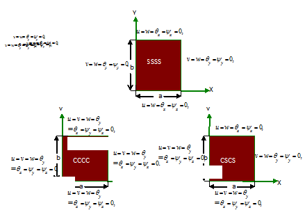
Figure 2 Schematic Diagram of Various Boundary Conditions.
The plate geometry used is characterized by aspect ratios (a/b) = 1and 2, side to thickness ratios (a/h) = 20, 30, 40, 50, 60, 80 and 100. The following material properties are used for computation Shen:12
Validation study for mean and random transverse
central deflection
Validation study for mean transverse central deflection
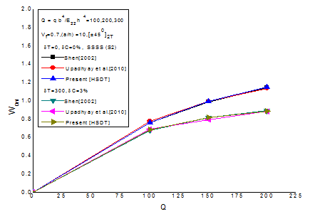
Table 1 compares the hygrothermal effects on the linear and non-linear bending behavior of a (±450)2T laminated square plate, dimensionless load deflection (Q) where (Q= q b4/E22h4=100, 150, 200), fiber volume fraction (Vf =0.6), plate thickness ratio (a/h =10), simple support SSSS (S2) boundary conditions and under environmental conditions. It is noticed that present [HSDT] result for mean hygrothermal deflection are in good agreement with the deterministic results of.12 Figure 3 compares the hygrothermal effects on the linear and non-linear bending behavior of a (±450)2T laminated square plate, dimensionless load deflection (Q) where (Q= q b4/E22h4=100, 150, 200), fiber volume fraction (Vf =0.6), plate thickness ratio (a/h =10), simple support SSSS (S2) boundary conditions and under environmental conditions. It is noticed that present [HSDT] result for mean hygrothermal deflection are in good agreement with the deterministic results of.12
(Q) |
Non-Dimensional Hygrothermal Bending Load |
Shen 12 |
Present[HSDT] |
Shen 12 |
Present[ HSDT] |
|
|
|
|
Non-linear |
Linear |
Non-linear |
Non-linear |
Linear |
Non-linear |
100 |
0.6887 |
1.328 |
0.6952 |
0.6261 |
0.9377 |
0.6222 |
150 |
0.8857 |
1.5801 |
0.883 |
0.7126 |
1.1067 |
0.7264 |
200 |
0.9909 |
1.7325 |
0.9989 |
0.777 |
1.1837 |
0.768 |
Table 1 Comparison of Hygrothermal Effects on the Linear and Non-linear Bending Behavior of a (±450)2T Laminated Square Plate, Load Deflection (Q) where Q= q b4/E22h4, Fiber Volume Fraction (Vf) =0.6, Plate Thickness Ratio (a/h) =10, Simple Support SSSS (S2) Boundary Conditions under Environmental Conditions


Figure 3 Validation study of dimensionless transverse central deflection of angle-ply square laminated composite plate subjected to linearly varying temperature.
Validation study for random transverse central deflection
Validation study for random hygrothermal central deflection of material properties (E22), plate thickness ratio (a/h) =30, aspect ratio (a/b) =1, rise in temperature
, rise in moisture concentration
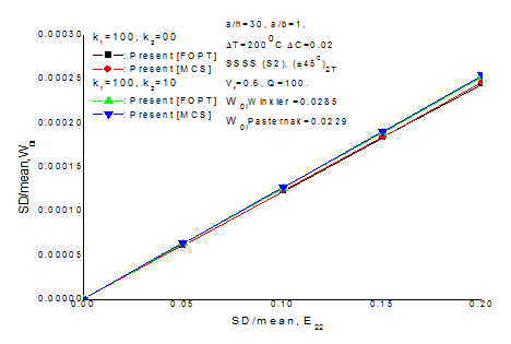
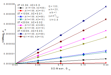
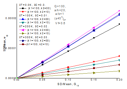
, simple support SSSS (S2), fiber volume fraction (Vf=0.6) , dimensionless load deflection (Q =100), angle ply antisymmetric (±450)2T laminated composite plate resting on Winkler (k1=100, k2=00) and Pasternak( k1=100, k2=10) elastic foundations is shown in Figure 4. It is seen that present FOPT results are satisfactory with the MCS results.
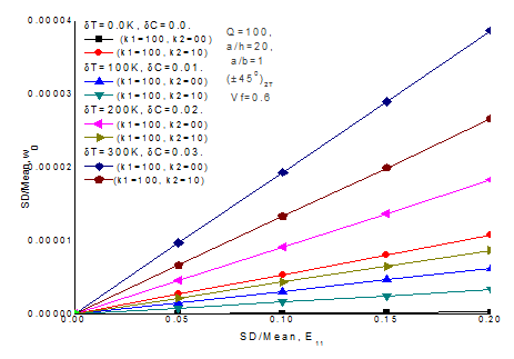
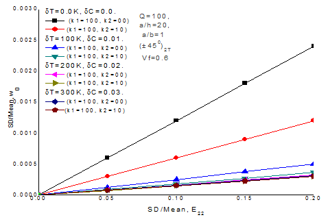
In (Table 2a) (Table 2b), it is observed that as increases the lateral pressure, the mean transverse central deflection increases and corresponding coefficient of variation decreases. It is noticed that expected mean transverse central deflection (W0l) value of individual random variables of hygrothermal deflection decreases for Winkler elastic foundation and it further decreases for Pasternak elastic foundation whereas COV of hygrothermal deflection increases on rise in temperature and moisture concentration as shown in Figure 5.
(bi) |
(k1=100, k2=00) |
|
|
|
|
COV, Wl, |
COV, Wl, |
COV, Wl, |
COV, Wl, |
|
(0.0351) 2.14e-07 |
(0.0312) 6.15e-06 |
(0.0273) 1.83e-05 |
(0.0234) 3.87e-05 |
|
0.0024 |
5.00E-04 |
3.27E-04 |
3.11E-04 |
|
5.06E-07 |
1.31E-06 |
3.35E-06 |
5.76E-06 |
|
1.81E-05 |
2.12E-05 |
2.26E-05 |
2.15E-05 |
|
9.08E-06 |
1.06E-05 |
1.13E-05 |
1.07E-05 |
|
7.19E-05 |
7.19E-06 |
4.77E-06 |
7.14E-06 |
|
1.53E-11 |
8.77E-11 |
1.58E-10 |
1.86E-10 |
|
4.05E-12 |
2.10E-10 |
6.75E-10 |
1.40E-09 |
|
7.42E-10 |
4.11E-08 |
1.31E-07 |
2.73E-07 |
|
6.76E-06 |
7.00E-06 |
7.32E-06 |
7.77E-06 |
|
0 |
0 |
0 |
0 |
|
2.52E-04 |
2.61E-04 |
2.73E-04 |
2.88E-04 |
Table 2(A) Effects of the Variation of Individual Random System Properties bi, [{(i =1 to 12), = 0.10] on the Dimensionless Expected Mean (W0l) and Coefficient of Variation (Wl) of Hygrothermomechanically Induced Central Deflection of Angle Ply (±450)2T Square Laminated Composite Plates Resting on Winkler (k1=100,k2=00) Elastic Foundations, Subjected to Uniform Constant Temperature and Moisture (U.T), in-plane Bi-axial Compression, Plate Thickness Ratio (a/h=20), with Simple Support S2 Boundary Conditions. The Dimensionless Mean Hygrothermal Deflections are given in Brackets. Load Deflection Q=100, Fiber Volume Fraction (Vf=0.6)
(bi) |
(k1=100,k2=10) |
|
|
|
|
COV, Wl, |
COV, Wl, |
COV, Wl, |
SD/Mean, Wl, |
|
(0.0330) 1.07e-05 |
(0.0291)3.26e-06 |
(0.0253) 8.63e-06 |
COV, Wl, |
|
0.0012 |
3.63E-04 |
2.98E-04 |
3.01E-04 |
|
1.03E-07 |
1.18E-06 |
2.68E-06 |
4.48E-06 |
|
7.42E-06 |
6.09E-06 |
2.43E-06 |
4.57E-06 |
|
3.71E-06 |
3.04E-06 |
1.21E-06 |
2.28E-06 |
|
0.0017 |
1.08E-04 |
1.20E-05 |
2.51E-07 |
|
2.03E-10 |
3.10E-10 |
4.21E-10 |
5.30E-10 |
|
2.17E-09 |
1.81E-09 |
1.39E-09 |
8.93E-10 |
|
4.16E-07 |
3.47E-07 |
5.82E-06 |
1.67E-07 |
|
5.63E-06 |
5.70E-06 |
5.82E-06 |
5.98E-06 |
|
5.29E-06 |
5.59E-06 |
5.79E-06 |
5.85E-06 |
|
2.52E-04 |
2.64E-04 |
2.78E-04 |
2.93E-04 |
Table 2(B) Effects of the Variation of Individual Random System Properties bi, [{(i =1 to 12), = 0.10] on the Dimensionless Expected Mean (W0l) and Coefficient of Variation (Wl) of Hygrothermomechanically Induced Central Deflection of Angle Ply (±450)2T Square Laminated Composite Plates Resting on Pasternak (k1=100, k2=10) Elastic Foundations, Subjected to Uniform Constant Temperature and Moisture (U.T), in-plane Bi-axial Compression, Plate Thickness Ratio (a/h=20), with Simple Support S2 Boundary Conditions. The Dimensionless Mean Hygrothermal Deflections are given in Brackets. Load Deflection Q=100, Fiber Volume Fraction (Vf=0.6)
For the same lateral pressure and temperature distribution, it is seen that the COV of transverse central deflection becomes more important as the plate thickness decreases i.e., a/h increases (Table 3). It is seen that on variations of thickness ratio the mean (W0l) hygrothermal deflection increases whereas COV of hygrothermal deflection decreases with different combinations of input random variables when laminated composite plates resting on Winkler and for Pasternak elastic foundations hygrothermal deflection decreases further with different combinations of input random variables in Figure 6.
a/h |
(k1=100, k2=00) |
(k1=100, k2=10) |
Mean, W0l |
Mean, W0l |
|
|
|
|
|
5 |
0.0126 |
0.0097 |
0.0304 |
0.0261 |
10 |
0.0278 |
0.0228 |
0.0314 |
0.0268 |
30 |
0.0377 |
0.0285 |
0.0338 |
0.0229 |
50 |
0.0411 |
0.0332 |
0.0351 |
0.0227 |
100 |
0.0449 |
0.0256 |
0.0364 |
0.0175 |
Table 3 Effects of Plate Thickness Ratios (a/h) with Random Input Variables bi, [{(i =1 to 9), (7..9), (10,11) and (12)} = 0.10] on the Dimensionless Expected Mean (W0l) of Hygrothermomechanically Induced Central Deflection of Angle Ply (±450)2T Square Laminated Composite Plates Resting on Winkler (k1=100,k2=00) and Pasternak(k1=100,k2=10) Elastic Foundations, Subjected to Uniform Constant Temperature (U.T), and In-plane Bi-axial Compression with Simple Support S2 Boundary Conditions. Load Deflection Q=100, Fiber Volume Fraction (Vf=0.6)
In Table 4, it is noticed that on increase of aspect ratio the mean (W0l) hygrothermal central deflection value increases for Winkler (k1=100,k2=00) and Pasternak(k1=100,k2=10) elastic foundations whereas COV of hygrothermal deflection decreases for all different combinations of input random variables, it is more dominant for Pasternak elastic foundations as shown in Figure 7.
a/b |
(k1=100, k2=00) |
(k1=100, k2=10) |
|
Mean, W0l |
Mean, W0l |
|
|
|
|
0.5 |
0.0027 |
0.0024 |
0.0024 |
0.0019 |
1 |
0.0395 |
0.0308 |
0.0345 |
0.0223 |
1.5 |
0.1947 |
0.1314 |
0.1562 |
0.1049 |
2 |
0.5555 |
0.3814 |
0.4088 |
0.29 |
Table 4 Effects of Aspect Ratios (a/b) with Random Input Variables bi, [{(i =1 to 9), (7..9), (10,11) and (12)} = 0.10] on the Dimensionless Expected Mean (W0l) of Hygrothermomechanically Induced Central Deflection of Angle Ply (±450)2T Square Laminated Composite Plates Resting on Winkler (k1=100,k2=00) and Pasternak(k1=100,k2=10) Elastic Foundations, Plate Thickness Ratios (a/h=40). Subjected to Uniform Constant Temperature (U.T), and In-plane Bi-axial Compression with Simple Support S2 Boundary Conditions. Load Deflection Q=100, Fiber Volume Fraction (Vf=0.6)
In Table 5 it is noticed that combined simple support and clamped support CSCS have significance effects on mean (W0l) hygrothermal deflection with different combinations of input random variables under environmental conditions. However the COV of hygrothermal deflection also varies accordingly under given environmental conditions and different combinations of input random variables for square composite plates resting on Winkler (k1=100,k2=00) and Pasternak(k1=100,k2=10) elastic foundations, mean and COV are significant for
Pasternak(k1=100,k2=10) elastic foundations as shown in Figure 8.
BCs |
(k1=100, k2=00) |
(k1=100, k2=10) |
Mean, W0l |
Mean, W0l |
|
|
|
|
SSSS (S1) |
0.0426 |
0.0346 |
0.0358 |
0.0232 |
SSSS (S2) |
0.0426 |
0.0345 |
0.0357 |
0.0231 |
CCCC |
0.0423 |
0.0411 |
0.0353 |
0.0358 |
CSCS |
0.0408 |
0.0686 |
0.0391 |
0.0777 |
Table 5 Effects of Support Conditions with Random Input Variables bi, [{(i =1 to 9), (7..9), (10,11) and (12)} = 0.10] on the Dimensionless Expected Mean (W0l) of Hygrothermomechanically Induced Central Deflection of Angle Ply (±450)2T Square Laminated Composite Plates Resting on Winkler (k1=100,k2=00) and Pasternak(k1=100,k2=10) Elastic Foundations, Plate Thickness Ratios (a/h=60). Subjected to Uniform Constant Temperature (U.T), and In-plane Bi-axial Compression with Simple Support S2 Boundary Conditions. Load Deflection Q=100, Fiber Volume Fraction (Vf=0.6)
In Table 6, it is observed that on change of lamina layup the mean (W0l) of hygrothermal central deflection decreases significantly for cross ply symmetric plate. The COV of hygrothermal central deflection also decreases for different combinations of input random variables. It is significant to note for cross ply symmetric plates with
and Pasternak elastic foundations as shown in Figure 9.
Lay-up |
(k1=100, k2=00) |
(k1=100, k2=10) |
Mean, W0l |
Mean, W0l |
|
|
|
|
(±450)2T |
(k1=100, k2=00) |
(k1=100, k2=10) |
(k1=100, k2=00) |
(k1=100, k2=10) |
(±450)S |
0.0335 |
0.0268 |
0.0302 |
0.0239 |
[00/900]2T |
0.0226 |
0.0178 |
0.0202 |
0.0156 |
[00/900] S |
0.0107 |
0.0088 |
0.0101 |
0.0082 |
Table 6 Effects of Lay-Up with Random Input Variables bi, [{(i =1 to 9), (7..9), (10,11) and (12)} = 0.10] on the Dimensionless Expected Mean (W0l) of Hygrothermomechanically Induced Central Deflection of Angle Ply (±450)2T Square Laminated Composite Plates Resting on Winkler (k1=100,k2=00) and Pasternak(k1=100,k2=10) Elastic Foundations, Plate Thickness Ratios (a/h=50). Subjected to Uniform Constant Temperature (U.T), and In-plane Bi-axial Compression with Simple Support S2 Boundary Conditions. Load Deflection Q=100, Fiber Volume Fraction (Vf=0.6)
In Table 7, it is seen that on increasing load deflection the mean (W0l) hygrothermal central deflection increases in given environmental conditions and different combinations of input random variables .The central deflection value and COV of hygrothermal central deflection decreases in similar conditions and important to note for plates with
and Pasternak elastic foundations as shown in Figure 10.
(Q) |
(k1=100, k2=00) |
(k1=100, k2=10) |
Mean, W0l |
Mean, W0l |
|
|
|
|
100 |
0.0377 |
0.0285 |
0.0338 |
0.0229 |
150 |
0.0563 |
0.0476 |
0.0501 |
0.0392 |
200 |
0.0698 |
0.063 |
0.0616 |
0.0523 |
Table 7 Effects of Load Deflections (Q) with Random Input Variables bi, [{(i =1 to 9), (7..9), (10,11) and (12)} = 0.10] on the Dimensionless Expected Mean (W0l) of Hygrothermomechanically Induced Central Deflection of Angle Ply (±450)2T Square Laminated Composite Plates Resting on Winkler (k1=100,k2=00) and Pasternak(k1=100,k2=10) Elastic Foundations, Plate Thickness Ratios (a/h=30). Subjected to Uniform Constant Temperature (U.T), and In-plane Bi-axial Compression with Simple Support S2 Boundary Conditions. Fiber Volume Fraction (Vf=0.6)
In Table 8, it is noticed that on varying fiber matrix volume fraction the mean (W0l) hygrothermal central deflection increases in given environmental conditions and different combinations of input random variables whereas the value of COV of hygrothermal central deflection also varies in similar conditions. It is to be noted for Pasternak elastic foundations and plates with
as shown in Figure 11.
(Vf) |
(k1=100, k2=00) |
(k1=100, k2=10) |
Mean, W0l |
Mean, W0l |
|
|
|
|
0.50 |
0.0381 |
0.0289 |
0.0332 |
0.0209 |
0.55 |
0.0385 |
0.0296 |
0.0336 |
0.0213 |
0.60 |
0.0395 |
0.0308 |
0.0345 |
0.0223 |
0.65 |
0.0413 |
0.0327 |
0.0361 |
0.024 |
0.70 |
0.044 |
0.0355 |
0.0385 |
0.0265 |
Table 8 Effects of Fibre Volume Fractions (Vf) with Random Input Variables bi, [{(i =1 to 9), (7..9), (10,11) and (12)} = 0.10] on the Dimensionless Expected Mean (W0l) of Hygrothermomechanically Induced Central Deflection of Angle Ply (±450)2T Square Laminated Composite Plates Resting on Winkler (k1=100,k2=00) and Pasternak(k1=100,k2=10) Elastic Foundations, Plate Thickness Ratios (a/h=40). Subjected to Uniform Constant Temperature (U.T), and In-plane Bi-axial Compression with Simple Support S2 Boundary Conditions. Load Deflection (Q)=100
In Table 9, it is noticed that on increasing temperature and moisture the mean (W0l) hygrothermal central deflection decreases in given environmental conditions and different combinations of input random variables whereas the value of COV of hygrothermal central deflection increases in similar conditions as noticed for plates with
and Pasternak (k1=100,k2=10) elastic foundations as shown in Figure 12.
Environmental conditions |
(k1=100, k2=00) |
(k1=100, k2=10) |
W0l |
W0l |
|
0.0533 |
0.0488 |
|
0.0486 |
0.0438 |
|
0.0436 |
0.0388 |
|
0.0384 |
0.0338 |
|
0.033 |
0.0288 |
|
0.0276 |
0.0238 |
Table 9 Effects of Temperature and Moisture Rise
with Random Input Variables bi, [{(i =1 to 9), (7..9), (10,11) and (12)} = 0.10] on the Dimensionless Expected Mean (W0l) of Hygrothermomechanically Induced Central Deflection of Angle Ply (±450)2T Square Laminated Composite Plates Resting on Winkler (k1=100,k2=00) and Pasternak(k1=100,k2=10) Elastic Foundations, Plate Thickness Ratios (a/h=20). Subjected to Uniform Constant Temperature (U.T), and In-plane Bi-axial Compression with Simple Support S2 Boundary Conditions. Load Deflection (Q)=150, Fiber Volume Fraction (Vf=0.6)
Conclusion
A C0 SFEM probabilistic procedure is adopted to compute the second order statistics of transverse central deflection of geometrically linear laminated composite plate in the framework of HSDT with randomness in material properties, coefficients of thermal expansion and coefficients of hygroscopic expansion, elastic foundation parameters and lateral loading.
Among the different system properties studied, the elastic moduli, elastic foundation parameters, lateral loading and environmental conditions have dominant effect on the COV of the transverse deflection when compared to other system properties subjected to uniform and linearly varying temperature distribution. In order to assess the effects of temperature and moisture on the bending behavior of shear deformable laminated plates, a theoretical analysis is developed based on a micro mechanical model.
The COV of the hygrothermomechanically induced transverse central deflection of the plate increases as distribution in lateral pressure increases, this bring out importance of considering hygrothermomechanical loading along with lateral pressure from design point of view specially in aerospace and other sensitive application where reliability of the components is important. Tight controls of these properties are therefore required for high reliability of the plate design. The flexural response of the laminated composite plate deteriorates considerably with the increase in temperature and moisture concentration and this hygrothermal environment becomes more detrimental as the working temperature reaches higher temperature.
Appendix
; (i,j=1,2,6)
; (i,j=4,5)
;
.
where
,
,
,
Where
Acknowledgements
Conflicts of interest
Author declares that there is no conflict of interest.
References
- Shen Hui. Nonlinear analysis of composite laminated thin plates subjected to lateral pressure and thermal loading resting on elastic foundation. Composite Structures. 2000;49(2):115‒128.
- Huang NN, Tauchert TR. Large deformation of anti-symmetric angle-ply laminated composites resulting from non-uniform temperature loading. J Thermal Stresses. 1998;11(3):287‒297.
- Shen Hui Shen. Nonlinear bending analysis of unsymmetric cross-ply laminated plates with piezoelectric actuators in Thermal environment. Composite Structures. 2004;63(2):167-177.
- Lin RM, Lim MK, Du H. Large deflection analysis of plates under thermal loading. Comput Meth Appl Mechanics Engng. 1994;117(3‒4):381‒390.
- Shen Hui Shen. Non-linear bending of shear deformable laminated plates under lateral pressure and thermal loading and resting on elastic foundations. J Strain Anal Eng Des. 2000;35(2):93‒108.
- Whitney JM, Ashton JE. Effect of Environment on the Elastic Response of Layered Composite Plates. AIAA Journal. 1971;9(9):1708‒1713.
- Adams DF, Miller AK. Hygrothermal micro stress in unidirectional composite exhibiting inelastic materials behavior. Journal of Composite Materials. 1977;11(3):285‒99.
- Lee SY, Chou CJ, Jang JL, et al. Hygrothermal effects on the linear and nonlinear analysis of symmetric angle-ply laminated plates. Composite Materials. 1992;21(1):41‒48.
- Sai Ram KS, Sinha PK. Hygrothermal effects on the bending characteristics of laminated composite plates. Computers & Structures. 1991;40(4):1009‒1015.
- Patel BP, Ganapathi M, Makhecha DP. Hygrothermal effects on the structural behavior of thick composite laminates using higher-order theory. Composite Structures. 2002;56(1):25‒34.
- Shen Hui Shen. Hygrothermal effects on the post buckling of shear deformable laminated plates. Int J Mech Sci. 2001;43(5):1259‒1281.
- Shen HS. Hygrothermal Effects on the Nonlinear Bending of Shear Deformable Laminated Plates. Journal of Engineering Mechanics. 2002;128(4):493.
- Salim S, Yadav D, Iyengar NGR. Analysis of composite plates with random material characteristics. Mechanics Research Communications. 1993;20(5):405‒14.
- Singh BN, Iyengar NGR, Yadav D. A C0 finite element investigation for buckling analysis of composite plates with random material properties. Int J Struct Engrg Mech. 2000;13:53‒74.
- Onkar AK, Yadav D. Non-linear response statistics of composite laminates with random material properties under random loading. Composite Structures. 2003;60(4):375‒383.
- Yang J, Liew KM, Kitipornchai S. Stochastic analysis of compositionally graded plates with system randomness under static loading. Int J Mech Sci. 2005;47(10):1519‒1541.
- Upadhyay AK, Pandey Ramesh, Shukla KK. Nonlinear flexural response of laminated composite plates under hygro-thermo-mechanical loading. Communications in Nonlinear Science and Numerical Simulation. 2010;152(9):2634‒2650.
- Lal A, Singh BN, Kumar Rajesh. Stochastic nonlinear bending response of laminated composite plates with system randomness under lateral pressure and thermal loading. Archive of Applied Mechanics. 2011;81(6):727‒743.
- Lal A, Singh BN. Effect of random system properties on bending response of thermo-mechanically loaded laminated composite plates. Applied Mathematical Modelling. 2011;35(12):5618‒5635.
- Kumar Rajesh, Patil HS, Lal A. Hygrothermal effects on the flexural response of laminated composite plates with random material properties: Micromechanical (SFEM) model. International Journal of Applied Engineering and Research (RIP). 2011.
- Kumar Rajesh, Patil HS, Lal A. Nonlinear Flexural Response of Laminated Composite Plates on a Nonlinear Elastic Foundation with Uncertain System Properties under Lateral Pressure and Hygrothermal Loading: Micromechanical Model. International Journal of Aerospace Engg. 2014;27(3):168.
- Reddy JN. A simple higher order theory for laminated composite plates. Trans ASME J Applied Mech. 1984;51(4):745‒752.
- Reddy JN. Mechanics of laminated composite plates. 2nd edn. Theory and Analysis, CRC Press, Florida, USA; 1996. p. 858.
- Kleiber M, Hien TD. The stochastic finite element method. John Wiley & Sons, USA; 1992. p. 322.
- Chia YA. Nonlinear analysis of plates. McGraw-Hill, New York, USA; 1980. p. 436.
- Shankara CA, Iyengar NGR. A C0 element for analysis of laminated composite plate. Journal of Sound and Vibration. 1996;191(5):721‒738.
- Jones RM. Mechanics of Composite Materials. 2nd edn. McGraw-Hill, Taylor & Francis group, USA; 1998. p. 538.
- Zongeen Z, Suhaun C. The standard deviation of the eigen solutions for random multi degree freedom systems. J Comp Struct. 1990;39(6):603‒607.
- Zhang Y, Chen S, Liu Q, et al. Stochastic perturbation finite elements. Computers & Structures. 1996;59(3):425‒429.
- Liu WK, Ted B, Mani A. A random field finite elements. Int J Numer Meth Engrg. 1986;23(10):1831‒1845.
- Zhang J, Ellingwood B. Effects of uncertain material properties on structural stability. J Struct Engrg. 1993;121(4):705‒716.
- Singh BN, A Lal, R Kumar. Nonlinear bending response of laminated composite plates on nonlinear elastic foundation with uncertain system properties. Engineering Structures. 2008;30(4):1101‒1112.
- Dash Padmanav, Singh BN. Geometrically nonlinear bending analysis of laminated composite plate. Commun Nonlinear Sci Numer Simulat. 2010;15(10):3170‒3181.
- Lal A, Singh BN, Soham Anand. Nonlinear bending response of laminated composite spherical shell panel with system randomness subjected to hygro-thermo-mechanical loading. International Journal of Mechanical Sciences. 2011;53(10):855‒866.
- Singh BN, Grover Neeraj. Stochastic Methods for the Analysis of Uncertain Composites. Journal of the Indian Institute of Science. 2013;93(4).

©2017 Kumar. This is an open access article distributed under the terms of the,
which
permits unrestricted use, distribution, and build upon your work non-commercially.


