In aircraft engines, one of the main goals is to decrease fuel consumption while minimizing design time and cost. The attachment between the blade and disc is a critical region of the turbine as it is subjected to high stress due to centrifugal and thermal loads that are transferred between these two components. Failure of this region can lead to critical engine failure. In this paper, a design optimization framework of the turbine blade and disc attachment, called fixing, is presented. The objective function of the optimization is to minimize the weight of the fixing while ensuring that stresses are in safe limits to avoid mechanical failure. For the optimization, in-house tools of Pratt & Whitney Canada will be used. Firstly, a Design and Analysis (D&A) tool will be used that combines Computer Aided Design (CAD) and Finite Element Analysis (FEA) commercial software running in batch mode. Furthermore, a Surrogate Assisted Optimization (SAO) tool will be used to explore the design space and find the optimum design. An in-house code has also been created that links the D&A and SAO tools. After the optimization framework was set up, a Design of Experiment (DOE) was used to create a sample of fixing configurations and a sensitivity analysis was implemented based on this sample. The results of the sensitivity analysis showed which geometric parameters have the greatest impact on the stresses applied on a fixing. Only the sensitive parameters were chosen to be optimized. The goal of this paper is to create an automated optimization tool that will increase the accuracy and decrease the time of the pre- detailed design process.

D&A       Design & Analysis

CAD       Computer Aided Design

FEA        Finite Element Analysis

SAO        Surrogate Assisted Optimization

CFD        Computational Fluid Dynamic

MDO      Multi-disciplinary Design Optimization

PMDO   Preliminary Multi-disciplinary Design Optimization

GUI        Graphical User Interface

GA          Genetic Algorithm

DOE       Design of Experiment

The design of an aeronautical gas turbine involves not only designing multiple components but also combining tools and engineering disciplines to create the optimum turbine for the design conditions. The design of a turbine’s components is consisted of two design phases: the pre-detailed or preliminary design phase and the detailed design phase. During the pre-detailed design phase a rough shape of the components has to be designed within limited time. The designers don’t have much knowledge available in the preliminary stage, so a compromise has to be done between the fidelity of the designs and the time needed to achieve them. During the detailed design phase more emphasis is given to the fidelity of the designs, more time is dedicated and more knowledge is available. Therefore, more accurate but usually slower methods such as Finite Element Analysis (FEA) and Computational Fluid Dynamic (CFD) are used to obtain the final design. The approach used in this phase is multi-disciplinary as different disciplines associated with engine design such as aerodynamics, stress, cooling, acoustics etc. are combined together so that an optimized solution is reached. Optimization using this approach is called Multi-disciplinary Design Optimization (MDO). However, during the detailed design phase there is almost no freedom to modify any part of the design. This can be seen in Figure 1, where percentage of the freedom of changing the design variables and the available knowledge to make a decision on design variables is plotted against the time stages. From what is shown by the solid lines, the knowledge increases almost exponentially while the design freedom decreases.

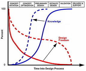
Figure 1 Knowledge and design freedom during the design process.¹

As anyone could understand, the preliminary design phase has a significant impact on the whole design process as it sets the technical envelope of the product. A false conception during the first stage, could mean a complete restart of the design process during the detailed design phase. Therefore, this design process has a major disadvantage which may lead to major delays in the planning and a rise of design costs. Applying Multi-disciplinary Design Optimization (MDO) at the preliminary design phase (PMDO) can eliminate the aforementioned problem. Specifically, it would allow investing more effort by incorporating cross-disciplinary knowledge earlier in the design process and thus increasing the available knowledge at the pre-detailed design phase as shown by the blue dotted line in Figure 1. It would also increase the design freedom as shown by the red dotted line in Figure 1. The integration of MDO in the pre-detailed stage would prevent the selection of an unsatisfactory concept early in the design process. This would result in the reduction in cost as it can be seen in Figure 2.

Figure 2 Cost committed during the design process.¹

As part of Pratt & Whitney Canada (PW&C) program on Propulsion System Integration and Optimization an integrated and automated turbine design and optimizer system is to be created by applying the PMDO approach. This design system will include the design of the platform, blade and disc attachment called fixing, disc, cover plate and airfoil based on mechanical and thermal stresses, aerodynamic and cooling requirements. The implementation of PMDO generally includes the following steps: parameterization of geometric and performance parameters, integration of disciplines and components and at last optimization. Until the current thesis several steps have been completed towards the creation of this system. The overall framework of this turbine design system has been created by Twahir et al.,¹ and it can be seen in Figure 3,^2,3 an automated design process of the airfoil has been developed by Doran et al.,⁴ Moradi et al.⁵ optimized the turbine gas-path etc.

Twahir et al.,¹ introduced the solution of incorporating CAD and FEA software in the pre-detailed design stage to significantly reduce the time of the design process of the turbine rotor fixing while ensuring accuracy. To improve this Design & Analysis (D&A) tool an optimization framework employed should be developed to provide an optimum design of the fixing to the pre-detailed design engineers. As a result, the risk of changing the design at the detailed phase would be eliminated and cost and time of design progress would be further reduced. Therefore, the current paper aims to create the aforementioned optimization framework.

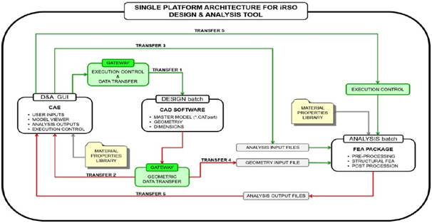
Figure 3 Single Platform Architecture for integrated Rotor System Optimizer (iRSO).¹

The D&A tool for fixings will be incorporated into the optimization framework to design and analyze the configuration created in each iteration. This tool will combine CAD and FEA tools that are usually set aside during the preliminary design stage. The user is able to both design and analyze a fixing from one Graphical User Interface (GUI). However, for the purpose of this study the batch version of this tool without the GUI will be used. The communication between the CAD and FEA software is driven by a CAE Gateway program. The user provides two input files, one file with all the geometric data to design a fixing and a second file with all the required mechanical parameters of the turbine required to analyze the fixing. These mechanical parameters are the centrifugal loads of the airfoil and the platform, the rotational speed of the rotor, the material of the blade and the disc, the temperature etc. The distribution of the centrifugal loads applied on the fixing among its parts is also included in the second input file. For example, for a three-lobe fixing the loads are shared among the Top, Middle and Bottom part as it can be seen in Figure 4. The load share depends on the shape of the fixing and as a result it changes in every iteration of the optimization process as a new configuration is tested.

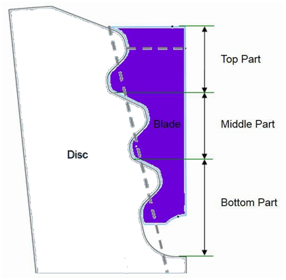
Figure 4 Three-Lobes fixing sections.²

The geometric data are transferred by the CAE to the CAD program. Then, a parameterized model, built in CATIA, is updated according to the given geometric parameters. The centrifugal load of the platform is recalculated as its shape is dependent on the shape of the top part of the fixing. This model, together with other user inputs, is sent to the FEA program to run a 2D stress analysis and recalculate the load share among the fixing. Afterwards, the centrifugal load applied on the fixing due to its rotated mass is calculated. At last, 1D stresses are calculated based on the updated load share, the 2D peak stresses are fetched by CAE from FEA and 3D stresses are estimated based on the 2D stresses. Output files are created including a file with the value stresses and loads, a CATIA model of the fixing according to the input geometric parameters and stress contours created by ANSYS. The workflow of the process described above is shown in Figure 5.

Figure 5 Workflow of D&A tool running in batch mode.

Parameterized model

In order to create a robust optimization framework, a very flexible and versatile parameterized model is very significant. However, a compromise between the flexibility of the model and the time needed for the parameterized model to be updated should be made as the goal of this framework is to reduce pre-detailed design time. Different seed CAD models are created in CATIA software for different multi-lobe fixings. The parameters of the CAD models are identical; however there are more parameters in the two-lobe model than in the one lobe and even more in the three and four-lobe models. For the development of the optimization framework only two and three-lobe fixings will be used. In addition, the three-lobe model will be used as an example in order to explain the parameterization method. This model geometry is divided into the three sections that were shown in Figure 4. Therefore, each section has a pair of a lobe and a neck. The two-lobe geometry is divided into two sections by losing the middle part.

The parameters that define the blade and disc part of the fixing can be explained by looking at a neck-lobe pair. Both the neck and the lobe are defined by the radius of 2 arcs and the length of a straight line that joins the two arcs tangent to both. The radius of the arc at the top part is referred to as the high radius, the radius of the arc at the bottom part is referred to as the low radius and the length of the line as side length. The straight line is also defined by an angle, called side angle. Between a neck and a lobe there is a straight line called bearing flat. This line is where the blade and disc portions of the fixing meet and therefore load flats. The length of this flat line and its angle, called load angle, define where the lobe is with respect to the neck. All the above parameters are shown in Figure 6.

Figure 6 The parameters defining the Neck-Lobe pair.²

At the bottom of the blade section the last lobe is connected with the horizontal line which is the bottom edge of the blade by. When a blade is riveted, there is the arc of the rivet radius at the bottom edge and a horizontal line while the height above this line is the rivet depth. These three parameters are shown in Figure 7.

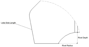
Figure 7 The parameters defining the blade bottom part.²

At the bottom part of the disc section of the fixing, after the last lobe, there is the live rim geometry. This geometry consists of two arcs, the top one called live rim high arc and the bottom one called live rim low arc. The radii of these two arcs and the distance between the bottom of the disc and the live rim, called live rim clearance, define the radius of this section of the disc. The geometry can be seen in Figure 8.

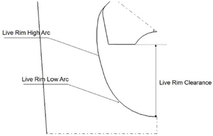
Figure 8 The live rim geometry at the bottom part of the disc.²

As the goal of this study is also to optimize the fixing of cooled blades as well the parameters needed to define the cooling area are presented. The user is able to define the number of cooling holes, the distribution among them and a few other parameters. For the purpose of this study, all the parameters defining the cooling passage of a fixing will remain constant and will be not optimized. However, the shape of the fixing of cooled blades will be optimized. In Figure 9 an example of a cooling configuration along with the parameters used to define it is presented.

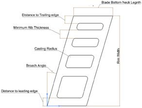
Figure 9 The parameters defining the cooling configuration.²

Stress analysis

Once the parameterized CAD model in CATIA is updated a 2D stress analysis runs on ANSYS and a recalculation of the load share among the parts of the fixing takes place. As the whole tool is running in batch mode, ANSYS also needs to run with no direct user input. This can be achieved by the FEA design language, which is a scripting language based on FORTRAN routines. This language also provides the ability to record sequences of FEA package commands in macro files. Several of these macro files are used to run FEA from the pre-processing to the solving to the post-processing. The meshing of the geometry is highly significant as it affects the results of the 2D stress analysis. A finer mesh should be used close to the critical regions such as bearing surfaces, blade necks and around live rim compared to the rest of the geometry. With this way, a high number of nodes will exist at the areas of interest while maintaining the amount of running time in a reasonable level. To achieve this, a minimum element size is set to provide a fine mesh around the critical regions and an expansion factor and expansion rate from one element to another is chosen. Like that, a smooth transition between the two meshes is secured. Regarding boundary conditions, the two bearing surfaces are coupled in the normal direction with displacement at zero. This condition reflects the behavior of the physical model, as the bearing surface of the blade section of the fixing may slide tangentially to the bearing surface of the disc fixing but cannot move normally. In addition, the nodes that are at the same radial position on the left and right edge of the disc section of the fixing are coupled in both tangential and normal direction. This comes from the fact that only a segment of the full disc is modeled so it cannot move tangentially or radially independently. The centrifugal loads due to rotation of the blade and the platform are modeled as the mass associated with the force at the specified rotational speed spread over the length of the top of the blade.

Based on the updated load share the 1D stresses are calculated. It is also assumed that the fixing is statically loaded and in equilibrium. For the 1D Analysis the direct, bearing, shear and bending stress are calculated. However, the final goal of the optimization is to evaluate the various configurations of the fixing based on 3D stresses. , the computational cost and time to run a 3D stress analysis in ANSYS in every iteration of the optimization process would be very high and it would not serve the goal of this optimization tool to deliver an optimum design in reduced time and cost. Thus, an estimation of the 3D stress based on the 2D stress results from ANSYS will take place instead of a fully 3D stress analysis. An estimation factor Kt2→3 is used to predict the 3D stresses acting on fixing based on the 2D stress results from ANSYS. This factor is a combination of a factor based on the broach angle of the fixing and another independent factor, whose value is calibrated so that the estimated 3D stresses are predicting the real 3D stresses with a significant accuracy. The estimation error, which is the difference between the predicted 3D stresses and the real 3D stresses, is less than 0.7% proving the validity of the prediction. The configuration of the fixing created in each iteration of the optimization process is, firstly, evaluated by 1D stresses and at a final stage by the 3D stresses.

Design optimization framework

As it was mentioned before, the region of the blade and disc attachment of a turbine, referred to as fixing, has a great impact on the operation of the turbine engine due to high stress acting on it. Extensive researches have been carried out in recent years in order to find the optimum design of the fixing using various optimization algorithms and software. In 2012 Hahn & Cofer⁶ firstly used a surrogate model based on Optimal Latin Hypercube approximation method using tools of Isight. In the second step, after identifying the most sensitive design variables, several optimization methods such as the NSGA-II non-dominated sorting genetic algorithm, Downhill Simplex and an evolutionary optimization algorithm were used and compared. Deqi Yu et al.,⁷ used the Multi-island genetic algorithm in order to obtain the optimal fir-tree root with better stress distributions and low stress concentrations. A single objective Genetic Algorithm (GA) was used by Alinejad et al.,⁸ in order to find the optimum fir-tree shape having minimum von- Mises stress.

In the current thesis, a Design of Experiment (DOE) and Surrogate Assisted Optimization (SAO) method included in an in-house tool of Pratt & Whitney Canada are used. In order to achieve the development of an optimization framework for fixings, the above in-house tool needs, firstly, to be connected with the D&A tool described in the previous chapter. To achieve the connection between them, a python script was developed. After the optimization workflow was set up, a DOE followed by a sensitivity analysis was carried out in order to identify the geometric parameters of the fixing that have the most significant impact on the stresses applied on it. At last, two different optimization approaches are proposed and their results are compared. For the implementation of the proposed optimization approaches a three-lobe fixing of an uncooled blade of a low pressure turbine and a two-lobe fixing of a cooled blade of a low pressure turbine were used in order to minimize the centrifugal load applied on them due to their rotation, referred as pull.

A Surrogate Assisted Optimization method is used in this research in order to find the global optimum configuration of the fixing. In this case, the objective function of the SAO is to minimize the pull of the fixing. In order to achieve this, the geometric parameters of the fixing that are set as design variables are altered through the optimization process in order to evaluate various configurations. These design variables are referred to as factors. In order to avoid the creation of infeasible configurations, limits are set to some of these factors based on manufacturing criteria. While aiming to reduce the weight of the fixing, the optimum design should not exceed the stress limits of the material of the fixing. Therefore, constraints are set on 1D and 3D stresses. The pull of the fixing along with the 1D and 3D stresses are called responses.

In order to analyze and understand this optimization method the following SAO workflow is presented in Figure 10. The first step of the workflow is to read the user’s settings. It includes, among others, the number of learning points (n) that are analysed at each optimization cycle until convergence is met. The second step is to build the surrogate model for each constraint and objective. Once the surrogate models are built the optimum is located. In addition, 1000 points are sampled for the next optimization cycle. Of these 1000 points, the n best points are selected based on a function of interest. The purpose of this function is to intelligently explore the design space to converge as quickly as possible to a physically acceptable solution. The selected n points, which are the factors, will be analysed by the D&A tool. The results from the D&A tool are passed to the SAO workflow as the responses and they are the n solutions shown in the workflow. At last the objective is checked and if the selected convergence criteria is met the optimum solution has been found, if not the process repeats itself.

In order to send the factors of each iteration into the D&A tool and pass the stresses and the pull of the fixing back to the SAO, a python script is developed called fixing.py. A simplified optimization workflow including the fixing.py script is presented in Figure 11. After SAO has selected the value of each factor, fixing.py updates the geometric parameters of the 1st input file of D&A tool according to these values. After the design and the stress analyses of the fixing are completed, fixing.py creates a file in which saves the pull of the fixing and the stress results as responses. Then, the SAO workflow continues as described above.

The developed optimization framework is ready to be used in order to find the optimum design of the fixing. The geometry of the fixing however is very sensitive and some combinations of the values of these factors may lead to infeasible designs. In addition, in such a high-dimensional problem the correlations between the factors and the objective would be very difficult to find and the surrogate model would be very complicated. As a result, the process would not be robust and would not lead to a significant better design. To validate this hypothesis an SAO was implemented with all the geometric parameters as factors. The process was very time expensive and didn’t lead to significant reduction of the pull. In particular, the optimization process converged to an optimum design after 45 hours and the weight reduction was 0.3%. In order to reduce the dimensions of the problem and the creation of infeasible geometries a sensitivity analysis was run in order to identify the most significant parameters.

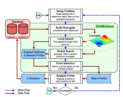
Figure 10 SAO workflow.⁴

Figure 11 Optimization framework.

Sensitivity analysis

The objective of the optimization process is to minimize the pull of the fixing while not exceeding the 1D and 3D stress limits of the material. In order to determine which geometric parameters have the greatest effect on the stresses, a sensitivity analysis should be performed. But firstly, the DOE method was used and then the results were evaluated by the sensitivity analysis. The type of DOE used in this case is a Latin Hypercube Sampling (LHS). The most common types of sensitivity analysis is gradient-based methods, such as local gradient, global mean gradient and global mean of absolute value of gradient. The first type does not account for interference effects or large perturbations and cannot be used for non-linear responses. The global mean gradient simply takes the mean of the gradient across the given region and the fatal flaw of this strategy is when a function is symmetric as the mean of the gradient is zero. The last type eliminates the symmetry issues but oscillatory or noisy functions will have a very large absolute mean even if the amplitudes are small. None of the gradient-approaches above can reliably define the relative impacts of each factor on each response. On the other hand, a variance-based sensitivity analysis can determine how much each response varies as each factor is varied across the sample in the design space and can deal with non-linear responses. The in-house tool used for the current sensitivity analysis is based on the last type. The 10 most influential factors were found for every response, which are the stresses and the pull of the fixing. In the Figure 12 an example of the results of the sensitivity analysis is presented. As it was expected, the radii and bearing flat of the top part of the fixing have the biggest impact on the bending stress. These graphics were created for every response of the optimization and all of them were examined to detect the most sensitive parameters of them. After detecting the geometric parameters that do not have a major impact on the stresses and the pull of the fixing, the SAO method, through the optimization framework that was previously described, is implemented by using only the sensitive parameters as factors.

Figure 12 Factors with highest impact on bending stress applied on top part of fixing’s disc section.

A three-lobe fixing of an uncooled blade of a low pressure turbine is firstly optimized. The material of the fixing is an alloy. After 24 hours, the optimization process concluded in an optimum design with a significant reduction of the pull of the fixing. In Figure 13 the shape of the blade section of the initial design is compared with the blade section of optimum fixing.

Figure 13 Initial and optimum design of the blade section of the fixing.

The centrifugal load applied on the optimum fixing due to its rotated mass, referred to as pull, was reduced by 27.71% compared to the pull applied on the initial configuration. This significant reduction will allow the reduction of the weight of the fixing by 27.7% leading to the potential of decreasing fuel consumption of the gas turbine. The 2D stress contour obtained by ANSYS of the initial design and the optimum one are compared in Figure 14. The stresses are in (psi) and as it can be seen, the stress distribution between the two designs is quite similar. The maximum 2D peak stress is located at the top part of the disc section of the fixing in both designs. As it was expected, the maximum peak stress of the optimum design is higher as its weight has been significantly reduced. However, the design is evaluated based on the 3D stresses. The maximum 3D peak stress applied on the design obtained by the optimization was augmented only by 1.14% compared to the initial design while still not exceeding the yield point of the material. The developed optimization framework can obtain an optimum design with a significant weight reduction and stress levels lower than the yield stress. This indicates the efficiency of the design optimization framework.

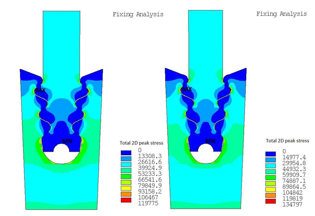
Figure 14 Comparison of 2D stress contour between the initial (left) and the optimum design (right).

However, in order to reduce the convergence time of the optimization process and thus the computational cost, a modified approach of the developed optimization framework was studied. This approach includes dividing the optimization on 3 steps. In the first step, the rough shape of the fixing will be optimized. After retrieving the optimum design of the above optimization, this design will be used as the initial one for the second step. In this step, more detailed parameters of the design will be optimized. The result of the second step will be used to optimize at last the least influential but still sensitive parameters of the fixing. This approach provides a better control of the optimization of the fixing and led to higher weight reduction in the same time compared to the optimization where all the sensitive parameters are optimized at once. The same initial design of the fixing was used to implement the 3-steps optimization. It is observed that the 3-steps optimization leads to greater pull reduction compared to one step optimization even from the 1st step. The overall convergence time is the same between the two approaches. However, the last step of the 3-steps optimization leads to an optimum design with a minor pull reduction of 0.15%. It is in the design engineers’ hands to decide if they want to dedicate 7 hours extra for this level of improvement. From the first two steps an optimum design of a great pull reduction is obtained in 17 hours, while with traditional pre- detailed design approach days were needed to conclude to a good first concept of the design. In Figure 15 the blade section of the fixing of the optimum design obtained after the last step of the 3-steps optimization is compared with the initial design. The overall reduction of the pull is 33.3%, while the one step optimization led to 27.7% reduction of the pull. As a result, it will allow to reduce the weight of the fixing even more.

Figure 15 Blade section of initial fixing compared with fixing obtained from 3-steps optimization.

In Figure 16 the 2D stress results from ANSYS of the optimum design are compared with  the initial one. As it was also observed in the previous optimization approach, the 2D stress is increased due to the pull reduction. The maximum 2D peak stress is again located at the top part of the disc section and specifically at the lobe of the fixing and the stress distribution between the two designs is similar. However, by looking on the maximum 3D stress, only an increase of 0.3% between the initial and the optimum design is observed. This augmentation is lower than the one when the initial fixing is compared to the fixing obtained from the one step optimization. Therefore, the 3-steps approach not only led to greater weight reduction in the same time, but also the maximum 3D stress remained almost the same. This proves the better robustness of the 3-steps approach.

A two-lobe fixing of a blade with cooling was used to implement the 3-steps optimization. In case of cooled fixing, the parameters that define the cooling passage remain constant and only the outer shape of the fixing is optimized. The number of the cooling passages is three and the air is distributed equally among them. After 23 hours the 3-steps optimization converged to the optimum design of the cooled fixing. It was expected that in the case of two-lobe fixing the convergence time would be lower as the optimized parameters are fewer. In Figure 17 the initial configuration of the blade section of the fixing is compared with the optimum configuration. The cooling passages of the blade section of the fixing remained the same.

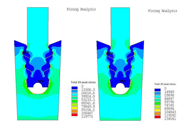
Figure 16 Comparison of 2D stress contour between the initial design (left) and the optimum design obtained from 3-steps optimization (right).

Figure 17 The initial and the optimum design of the blade section of a cooled fixing.

The pull of the fixing was reduced by 12.96%. As it can be seen in Figure 18, the stress distribution is similar in both designs and the maximum stress is located at the top lobe of the disc section of the fixing. Regarding the 3D stresses, the maximum 3D stress of the optimum fixing was augmented by 1.8% compared to the initial one. The greatest reduction of the pull of the fixing took place in the first two steps as it was reduced by 6.7% and 4.46% respectively.

This study presented the development of a framework to optimize the attachment of the turbine blade on the disc, called fixing. The objective of the optimization was to minimize the centrifugal load applied on the fixing due to its rotation, referred as pull. This reduction, in the next step, will allow the reduction of the weight of the fixing and thus will lead to a decrease of the engine’s fuel consumption. Two test cases were used to implement the optimization framework, a three-lobe fixing of a low-pressure turbine blade without cooling and a two-lobe fixing of the same blade with cooling. All the sensitive geometric parameters of the first test case were optimized in one step.  Results showed a 27.7% reduction of the pull of the fixing, a reduction of paramount importance. However, a modified approach of the implemented optimization framework was studied. The optimization process was divided into three steps. . This three-step approach was implemented for the first test case and it led to an optimum solution with 33.3% pull reduction, while the convergence time remained the same with the one step optimization. To validate the robustness of this modified approach, the second case was used to implement it. Results showed a significant reduction of 12.96%. The 1D and 3D stresses applied on the optimum solutions were all under the stress yield points of the material and compared to the according initial designs the stress’ increase did not exceed 1.8%. In addition, the optimum designs were validated by common practices used by aircraft engine manufacturing industries in order to assure that the structures will perform as intended in all aspects: form, function, producibility, durability and, above all, safety and reliability. During the 3-steps optimization process, after each step is completed, the factors and the initial design of the next step are changed manually. In order to automate the process, a python script was developed which updates the factors and the initial design between steps. The integration of an optimization method with CAD and FEA software into the pre-detailed design stage of turbine blade fixing led to a great reduction of its weight, contributing to the decrease of the engine’s fuel consumption. In addition, the automation of the design optimization process has also decreased the amount of time taken to achieve an optimum fixing.

Figure 18 Comparison of 2D stress contour between the initial (left) and the optimum design (right) of fixing with cooling.

None.

Authors declare that there is no conflict of interest.

1. Twahir A, Doré S, Moustapha H, et al. A Framework for an Integrated Turbine Rotor Design System. 1st Global Power and Propulsion Forum, GPPF-2017- 164: Zurich, Switzerland; 2017.
2. Twahir A, Roy F, Attia M, et al. Preliminary Design and Analysis Tool for Aeroengine Turbine Fixings. ASME International Mechanical Engineering Congress and Exposition, IMECE2014- 39039: Montreal, Quebec, Canada; 2014.
3. Twahir A. Preliminary Design of Blade and Disc Fixing for Aerospace Application using Multi-Disciplinary Approach. Master Thesis, Embry-Riddle Aeronautical University; 2013. 68 p.
4. Doran P, Vlasic E, Guevremont G, et al. Gas-path Optimization Using Turbine Aerodynamics Meanline and Design Exploration. Global Power and Propulsion Society, GPPS-2018- 0014: Montreal, Quebec, Canada; 2018.
5. Moradi N, Moustapha H. Rapid Airfoil Design for Uncooled High Pressure Turbine Blades. ASME Turbo Expo, GT2015-42514: Montreal, Canada; 2015.
6. Hahn Y, Cofer JI. Design Study of Dovetail Geometries of Turbine Blades Using Abaqus and Isight. ASME Turbo Expo, GT2012-68566: Copenhagen, Denmark; 2012.
7. Yu D, Li F, Yang J, Cheng K, et al. Structural Optimization of Fir-Tree Root and Groove for Turbine Blade with Splines and Genetic Algorithm. ASME Turbo Expo, GT2016-56518: Seoul, South Korea; 2016.
8. Alinejad F, Botto D, Gola M, et al. Reduction of Design Space to Optimize Blade Fir-tree Attachments. ASME Turbo Expo, GT2018-75781: Oslo, Norway; 2018.