This study investigates the feasibility of using Flush Air Data Sensing (FADS) System technology for air data measurements at the very low-airspeeds, where many Unmanned Aerial Vehicles (UAVs) operate. FADS is a non-intrusive alternative to pitot probes, where the vehicle nosecone, wing leading edge, or other aerodynamic surfaces are configured with multiple pressure-ports distributed along the windward face. Although FADS technology has been used for a variety of high-speed aircraft, FADS has never been applied to very low-airspeed flight regimes. This study reports on wind tunnel tests of two 3-D printed shapes: 1) a cylindrical body with a hemispherical head, and 2) a Rankine-Body. These body shapes can act as a vehicle analog to a wide range of three-dimensional shapes and account for both blunt leading edge and trailing after body flow characteristics. For this study the "probes" were printed with 5 pressure ports and the associated flow channels aligned at 0^o, +22.5^o and +45^o direction-angles along the vertical centerlines of the models. Sensed pressure data were curve-fit, developing quasi-potential flow calibration models for each probe, with coefficients compiled as a function of geometric angle-of-attack and tunnel airspeed. The calibration models account for end-to-end systematic effects, including the mounting sting flow compression, up wash, and tunnel blockage. Using the derived calibration models and the sensed pressure data, the effective angles-of-attack were re-calculated using the well-known "Triples" algorithm. The associated airspeed and dynamic pressure are estimated from the sensed pressure data using non-linear regression. The resulting estimates are compared to the tunnel reference conditions. Generally, both probe shapes performed well, with the redundant 5-port arrangement allowing for significant noise rejection. Both probes achieved RMS airspeed errors of less than 5%, angle-of-attack errors less than 1 deg., and dynamic pressure errors of less than 12 pascals, across airspeeds ranging from 5 to 25 m/sec. The sensed Airdata measurements at the lowest airspeeds (5 m/sec), exhibited similar accuracy to those sensed at the highest airspeeds (25 m/sec), verifying the applicability of FADS technology to very low airspeed flight regimes.

Keywords: UAV, low airspeed, air data, Rankine body, potential flow, FADS

A = quasi-Newtonian model slope fit coefficient; B = quasi-Newtonian model bias fit coefficient; 𝔸= triples solution parameter; 𝔹 = triples solution parameter; a = spherical radius, cm; b = source location, cm; = coefficient of pressure, and incidence angle; C_p = calculated FADS pressure coefficient vector; F = incidence angle function; i = port or pressure triples index; j = FADS solution algorithm iteration index; m = source strength; N = number of available pressure ports; n = non-linear Triples algorithm iteration index; n_T = number of available Triples; $\overline{n}$ = unit vector on body surface; $P_0$  = stagnation pressure, kPa; $P_{\theta }$ = local surface pressure at incidence angle, kPa; $P_{\infty }$ = freestream static (or ambient) pressure, kPa; $\overline{P}$ = sensed FADS pressure vector, kPa; $q_i$ = angle-of-attack averaging weighting parameters; $q_C$ = (compressible) dynamic pressure, kPa; R = polar radius coordinate, cm; r = Rankine-Body centerline radial coordinate, cm; u = longitudinal-axis airspeed, m/s; v = lateral-axis airspeed, m/s; $V_R$ = radial velocity component, m/s; $V_{\theta }$  = circumferential velocity component, m/s; $V_{\infty }$ Freestream flow velocity or airspeed, m/s; $\overline{V}$  = velocity vector, m/s; w = normal-axis airspeed, m/s; x = Rankine-Body centerline axial coordinate, cm; $\alpha$ = angle-of-attack, deg; ${\alpha }_e$ = effective aerodynamic angle-of-attack, deg; ${\alpha }_f$ = flank angle of attack, deg; $\widehat{\alpha }$ = mean effective angle-of-attack solution, deg; $\delta \alpha$ = systematic angle of attack calibration error, deg; $\beta$ = angle-of-sideslip, deg; $\epsilon$ = incidence angle scaling factor; ${\Gamma }_{u,c,L}$ = triples difference parameter; $\varphi$ = potential function, def. 1; $\varphi$ = clock angle, deg, def. 2

$\rho$ = air density, kg/m3; $\Theta$ = cone angle, deg; $\theta$ = surface incidence angle, deg; $\overline{\theta }$  = calculated FADS Incidence angle vector, deg; $\phi$ = Rankine-Body polar angle, deg; $V_{\infty }$ = freestream velocity, airspeed, m/s

The rapid development and deployment of Unmanned Aerial Vehicles (UAV) systems, commonly referred to as "drones," is potentially the most significant aviation development of the last 50 years. Applications include city and urban planning, land and resources management, law enforcement, mineral resource development, forest fire-prevention monitoring, agriculture, environmental monitoring, and military surveillance.¹ However, when compared to conventional aviation, many potential UAV missions are quite unconventional. The increased usage of UAVs in cities and residential areas requires flight through constrained space, and rapid maneuvering at high angles-of-attack to skirt around potential ground obstacles is an endemic part of the flight regime. UAV controllers relying on inertially-based sensors or GPS provide limited information on the actual mode of operation of the vehicle's aerodynamic surfaces (normal, stalled, spin), which can cause catastrophic losses of control when flying in turbulent weather conditions. Because of the need for high-rate feedback data, the effects of unsteady aerodynamics become potentially significant.

Thus, as described by Sankaralingham and Ramprasadh,² precise knowledge of airspeed and flow direction angles are particularly important for UAV flight. Collectively, the combination of airspeed, altitude, angle-of-attack, and -sideslip, and Mach number (for high-speed flight) are referred to as the "airdata state."³ Because this collection of parameters define wind-relative and local atmospheric conditions, it provides additional information not available from GPS or inertially-derived data. Sensing these parameters in real time allows a whole suite of control and stability-augmentation algorithms to be implemented. Such improvements can significantly enhance reliability and flight safety. This outcome may allow increased use of UAVs for deliveries, search and rescues, surveillances, and other commercial industries that, due to reliability or safety concerns, have not yet adopted the use of UAV.

Conventional aircraft use pitot-static probes and flow direction vanes to gather critical wind-relative flight information. As described by Gacey,⁴ for a typical aviation application, the air-data sensing system employs both pitot- and static pressure measurements that are sensed by a probe system. The angle-of-attack (α) and -sideslip (β) are sensed by flow direction vanes attached to the probe, with the pivot direction being sensed by a potentiometer or other bridge-based device. Figure 1 shows a typical airdata probe arrangement. The system is typically fuselage mounted with an extension that allows the airdata parameters to be sensed away from the influence of the body.

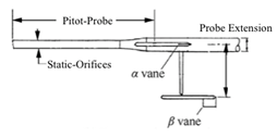
Figure 1 Conventional air data probe assembly.

When compared to the size of conventional aircraft, the sizes of the airdata probes of the form as shown by Figure 1 are sufficiently small so as not to change the overall vehicle flight dynamics. However; due to the small size and low wing loading of UAVs traditional probes have the potential to significantly change the vehicle flight dynamics, including an increase in parasitic drag, and a significant change in the weight-and-balance. Also, at the low-airspeeds and dynamic pressures associated with UAV flight, probes and booms are susceptible to vibration, can be easily damaged by rough vehicle landings, may have alignment issues due to the flexible structures, and require multiple moving parts, with the associated response dynamics. Thus, the development of an alternate, less intrusive, approach to airdata measurements for UAVs is highly desirable.

This project seeks to develop a smaller-sized, less-intrusive technology for UAV airdata measurements by leveraging Flush Airdata Sensing (FADS) technology. The FADS concept, where air data are inferred from non-intrusive surface pressure measurements, does not require probing of the local flow-field to compute air data parameters. Instead FADS uses the natural contours of the vehicle forebody or wing leading edge. This minimally-intrusive approach is ideal for UAV applications. Also, because the FADS system requires no moving parts, issues associated with dynamical response of the flow direction vanes and their associated potentiometer sensors do not exist.

As summarized by Ellsworth and Whitmore,⁵ the first major effort to collect air data on a hypersonic vehicle was the “Ball-Nose Flow Direction Sensor” on the X-15 rocket powered research vehicles in 1965.^6,7 This sensor consisted of 4 pressure ports attached to pressure transducers with the ports mounted on a moveable spherical nose cap. The sensor was steered to null the normal and lateral pressure port differences. By measuring the position of the ball at the nulled position, angles of attack and sideslip could be determined. The cumbersome analog system was prone to hydraulic failures, and was required to be dismantled and inspected between flights to insure integrity of the components. The Ball Nose Sensor was abandoned when the X-15 project concluded. The Shuttle Entry Air Data System (SEADS), Siemers et al.,⁸ used flush pressure ports on the shuttle nose cap that allowed gathering of in-flight windward pressure data Mach numbers significantly than could be gathered by the those shuttle's deployable hemispherical probe system. This preliminary concept was tested on a KC-135 in early 1981, Larson and Siemers.⁹ The SEADS was flight tested on the Columbia orbiter on Mission 61c, Henry et al.,¹⁰ In 1987, FADS at transonic speeds and high angles of attack was evaluated qualitatively on an F-14, Larson et al.,¹¹ to determine system performance for application to general aircraft under a large range of flight conditions. For these early programs, the sensed pressures were related to the desired airdata parameters using a nonphysical mapping. These tests verified the feasibility of the fixed orifice concept but did not demonstrate real time–capable algorithms for estimating the airdata from the pressure measurements.

The first estimation algorithms capable of real-time operation were developed at the NASA Dryden flight research center during the late 1980’s for the F/A-18 High Alpha Research Vehicle (HARV) program. The HARV flight tests also demonstrated that the measurement range of FADS systems could be extended to angles of attack greater than 60°. The computations were performed post flight using pressure data telemetered to the ground. Whitmore and Moes.^12,13 Failure detection and fault management methods were developed in the early 1990’s for the same system. Whitmore and Moes,¹⁴ The FADS approach was adapted for installation on a wing leading edge in 1993 by Whitmore an Czerniejewski.¹⁵ This design option allowed for the operation of a FADS system that would not interfere with the fire-control radar system in military vehicles. An analysis of the feasibility and uncertainty associated with using a FADS system under hypersonic conditions was added in 1994, Whitmore.¹⁶ In 1995, The estimation algorithms developed for the HARV program were demonstrated in a real-time flight environment on the NASA Dryden F/A-18 Systems Research Aircraft (SRA), Whitmore et al.,¹⁷ Up to this point, all of the FADS system calculations were performed post flight, and compared with other telemetry data. Cobleigh, et al.,¹⁸ expanded the calibration technique to apply to generic blunt fore bodies in 1998. Crowther and Lamont,¹⁹ at the University of Manchester published a paper detailing their work on calibrating Neural Networks to interpret pressure data for an arbitrary fuselage design. At roughly the same time, Rohloff, et al. published similar work using neural networks to calibrate flush airdata systems for blunt-nosed configurations.^20,21

The FADS system was applied to three premier hypersonic flight programs in the late 1990’s, the X-33, X38, and X-43 hypersonic research vehicles. For the X-33 program, Whitmore et al.,²² designed and calibrated a FADS system using detailed wind tunnel test data was designed and calibrated in 1998. Unfortunately, the X-33 program was cancelled before the system could be flight-tested.²³ The X-38 system relied on FADS for control system feedback and gain scheduling.²⁴ The system was evaluated under subsonic flight conditions for multiple test flights conducted between 1996 and 1998. During one-drop test, angle-of-sideslip feedback from the FADS system allowed the control system to right the vehicle after it roll-departed following it release from the B-52 carrier aircraft. In 2000, Davis, et al.,²⁵ developed a FADS system for use at supersonic and hypersonic speeds for the X-43 Hyper-X Scramjet demonstration vehicle. The FADS system was intended for later use in the guidance of hypersonic wedge shaped vehicles. The X-43 system was flown as an experiment to demonstrate the feasibility of operating a FADS system on a sharp-nosed waverider configuration. Pressure data was obtained from launch to the impact for all three X-43 test flights, and the results were analyzed post flight. dream chaser flush airdata system. In 2017 a FADS system was developed and flight tested for the Sierra Nevada Corporation’s Dream Chaser Spaceplane.²⁶ For the second approach and landing test, the original nose boom was replaced with a FADS, designed to fly on the orbital vehicle. The FADS-derived airdata parameters were fed-back to the flight software for vehicle guidance and control.

FADS measurements at very low airspeeds

To Date the lion's share of all FADS development work was been for military-class high speed and hypersonic flight vehicles. Although the FADS concept has been proven to work well for high speed configurations where dynamic pressure levels are relatively high, very little development with regard to lower-speed applications has been performed. Recently, Laurence and Argrow²⁷ successfully adapted a FADS systems of a Small Unmanned Aerial System (UAS), the X-8 Skywalker. Computational fluid dynamics simulations were used to determine the port locations of the FADS. Airframe locations were sorted based on the total sensitivity over a range of angles of attack and sideslip. Multilayer feed forward neural networks were employed to produce estimates of the angle of attack and sideslip, while static and stagnation ports on the fuselage measured airspeed. Accurate results were reported for airspeeds as low as 25 m/sec. This airspeed, 25 m/sec, lies at the upper limit of where many emerging UAV systems will operate. Because FADS sensing methods rely on differential pressures to triangulate the incoming flow direction vector, the measurement accuracy is especially susceptible to sensor measurement noise. The low dynamic pressure levels associated with low-speed UAV flight regimes present a significant measurement challenge. Typical operating airspeeds for UAVs range between 5 and 45 kts, (5 - 20 m/sec). At these very low airspeeds, the associated pressure differences across windward surfaces are rather small, resulting in very poor signal-to-noise ratio.

In order to assess whether FADS technology can reliably measure airdata at very low airspeeds, this study reports on very low-speed wind tunnel tests of two 3-D printed forebody shapes: 1) a cylindrical body with a hemispherical head, and 2) a Rankine-Body. These body shapes will approximate a wide range of three-dimensional shapes, and will act as a vehicle analog, accounting for both blunt leading edge and trailing afterbody flow characteristics. For this study, only the angle-of-attack flow plane was investigated, and the "probes" were printed with 5 pressure ports and the associated flow channels along the vertical centerline, aligned at 0o, +22.5o and +45o angles relative to the incoming flow direction. For this analysis the well-known "Triples" algorithm as developed by Whitmore et al.,¹⁶ is used for the FADS solution. Follow-on work using machine-intelligence algorithms is proposed at the end of this report. Details of the wind tunnel model designs will be presented later in the "Test Systems" section of this report.

FADS measurement issues for the low-speed (UAV) flight regime

In order to illustrate the required accuracy levels, the pressure distributions on a simple Rankine-Body²⁸ are presented. The Rankine model is representative of a wide-range of three-dimensional forebody shapes, and accounts for both blunt leading edge flow characteristics and the trailing afterbody. Conveniently, the model allows the low-speed surface pressure distributions to be analytically predicted in three-dimensions for an incompressible flow field. The analytical methods for the Rankine forebody analysis are presented later in the "Theoretical Considerations" Section of this report. Figure 2 plots the continuous surface pressure distributions for a Rankine-Body, "flying" at sea level, with freestream velocities of 5 and 20 m/sec. Note that the total differential pressure levels across the forebody are very small, ranging between only 0.50 (0.24 millibars) and 8.1 lbf/ft² (3.9 millibars). Also plotted on these figures pressure "taps" that have been sampled at 5 different points along the Rankine-Body's vertical centerline. The sampled pressure data have been corrupted with a Gaussian-distributed white noise. The corrupted data are taken to be representative of data sensed by a bank of differential pressure transducers.

Figure 2 Rankine-Body surface pressure distributions at 5 m/sec and 20 m/sec airspeeds, corrupted by two different measure-error levels.

Figures 2(a)–2(d) plot these results. Here the Rankine-Body pressure curve is overlaid by the exact and corrupted sampled data points. Figures 2(a)&2(b) assume a noise standard deviation of approximately +0.5 lbf/ft² (0.024 kPa). Figures 2(c)&2(d) plot the same data, except now the assumed measurement accuracy is improved with the noise standard deviation being approximately +0.1 lbf/ft² (0.005 kPa). Figures 2(a)&2(c) correspond to 5 m/sec airspeeds, and Figures 2(b)&2(d) correspond to 20 m/sec airspeeds. Also, from the data of Figures 2 note that at higher airspeed 20 m/sec, the prescribed measurement accuracy ranges reasonably reproduce the Rankine-body pressure curve. However, for the lower airspeed 5 m/sec, the +0.5 lbf/ft² error level does a very poor job of reproducing the pressure curve, and the higher accuracy +0.1 lbf/ft² level reasonably reproduces the pressure curve. Thus, it appears that the measurement constraints at these low airspeeds are very stringent.

This study reports on low-speed wind tunnel tests of two 3-D printed shapes: 1) Cylindrical body with a hemispherical head, and 2) a Rankine-Body. These body shapes can act as a vehicle afterbody analog for a wide range of three-dimensional shapes. These shapes account for both blunt leading edge and trailing afterbody flow characteristics. Fortunately, the incompressible (low speed) flow file around these simple shapes can be analytically predicted. This characteristic greatly simplifies the supporting analysis necessary to complete this problem.  This section reviews the potential flow analysis for the steady-state flows around a hemisphere and a Rankine-Body.

Doublet in uniform flow, flow around a spherical body (stokes flow)

As described by Kuethe and Chow,²⁹ when a 3-dimensional doublet (source and sink of equal strength) is inserted into a uniform flow field with velocity V_∞, the resulting flow field takes the form of a spherical shape. shows the resulting streamlines. This flow field is often referred to as "Stokes Flow." Figure 3 shows this field, where, θ is the incidence angle between the local surface normal and the incoming uniform flow stream, R is the polar radius from the doublet center, and a is the radius of the resulting spherical streamline. The net massflow across the spherical stream line is zero, thus this streamline can be considered as a solid boundary. The associated potential function ϕ for the external flow has the form,

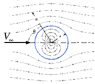
Figure 3 3-dimensional doublet in uniform flow (stokes flow filed).

$\varphi (R,\theta )=-V_{\infty }.a.\left[\frac{R}{a}+\frac{1}{2}.{\left(\frac{a}{R}\right)}^2\right].\cos \theta$   (1)

Calculating the velocity components,

$\overline{V}=-\overline{V}\varphi =\left[\begin{array}{l}{V}_R=-\frac{\partial }{\partial R}\varphi (R,\theta )=V_{\infty }.\left[1-\left(\frac{a^3}{R^3}\right)\right].\cos (\theta )\\ V_{\theta }=-\frac{1}{R}.\frac{\partial }{\partial R}\varphi (R,\theta )=-V_{\infty }.\left[1+\frac{1}{2}-\left(\frac{a^3}{R^3}\right)\right].\sin (\theta )\end{array}\right]$   (2)

On the surface of the sphere, the velocity components reduce to

$\begin{array}{l}{(}_{V_r}=V_{\infty }.\left[1-\left(\frac{a^2}{r^3}\right)\right].\cos \theta =0\\ {(}_{V_{\theta }}=-\frac{3}{2}{V}_{\infty }.\sin (\theta )\end{array}$   (3)

From Incompressible Bernoulli's Law, [29, pp. 63] the local surface pressure $P_{\theta }$ is related to the stagnation pressure $P_0$ by

$P_0=P_{\infty }+\frac{1}{2}\rho .V_{\infty }{}^2=P_{\theta }+\frac{1}{2}\rho .{(V_{\theta })}^2=P_{\theta }+\frac{1}{2}\rho .V_{\infty }{}^2\left(\frac{9}{4}{\sin }^2(\theta )\right)$   (4)

Solving for the local surface pressure coefficient,

$C_{P_{\theta }}\equiv \frac{P_{\theta }-P_{\infty }}{\frac{1}{2}\rho .V_{\infty }{}^2}=\left(\frac{P_{\theta }-P_{\infty }}{q_c}\right)=1-\left(\frac{9}{4}{\sin }^2(\theta )\right)=\frac{9}{4}{\cos }^2(\theta )-\frac{5}{4}$   (5)

In Eq. (5), $P_{\infty }$ is the freestream static pressure, and qc is the local (compressible) dynamic pressure.

Single source in uniform flow, flow around a Rankine-Body

In contrast, when only a single source is immersed in a uniform flow, the "Rankine-Body"^28,30 shape of Figure 4 results. The associated source location b, and strength are m,

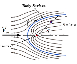
Figure 4 Source in uniform flow, Rankine-body flow field.

$\begin{array}{l}b=\frac{D}{2\pi }\\ m=2\pi .b.V_{\infty }\end{array}$   (6)

The corresponding potential function is

$\varphi (R,\phi )=V_{\infty }.\left[R.\cos \phi +\frac{D}{2\pi }.ln(R)\right]$   (7)

with a polar radius given by

$R=b.\frac{(\pi -\phi )}{\sin \phi }=\frac{D}{2\pi }.\frac{(\pi -\phi )}{\sin \phi }$   (8)

In Eqns. (6), (7), and (8), D is the body diameter, and   is the polar angle measured counterclockwise from the centerline of the resulting body. Calculating the velocity components,

$\overline{V}=\overline{V}\varphi \to \left[\begin{array}{l}{V}_R=-\frac{\partial }{\partial R}\varphi (R,\theta )=V_{\infty }.(\cos \phi +\frac{D}{2\pi }.\frac{1}{R}\\ V_{\theta }=-\frac{1}{R}.\frac{\partial }{\partial R}\varphi (R,\theta )=-V_{\infty }.\sin \phi \end{array}\right]$   (9)

Calculating the square of the velocity vector from Eq. (9),

$V^2=V_{\infty }{}^2\left[{\left(\cos \phi +\frac{D}{2\pi }.\frac{1}{R}\right)}^2+{\sin }^2\phi \right]=V_{\infty }{}^2\left[1+2.\frac{D}{2\pi .r}.\cos \phi +{\left(\frac{D}{2\pi .R}\right)}^2\right]$   (10)

and substituting into Bernoulli's Law,

$p_{\varphi }+\frac{1}{2}\rho .V_{\varphi }{}^2=p_{\infty }+\frac{1}{2}\rho .V_{\infty }{}^2\to C_{p_{\varphi }}=\frac{p_{\varphi }-p_{\infty }}{\frac{1}{2}\rho .V_{\infty }{}^2}=1-\left(\frac{V_{\varphi }}{V_{\infty }}\right)$   (11)

the local pressure coefficient on the surface of the body is

$C_{p_{\varphi }}=\frac{p_{\varphi }-p_{\infty }}{\frac{1}{2}\rho .V_{\infty }{}^2}=1-\left(\frac{V_{\varphi }}{V_{\infty }}\right)=1-\sin \phi$   (12)

The 2-D centerline body surface coordinates are given by

$\begin{array}{l}r=R.\sin \phi =\frac{b.(\pi -\phi )}{\sin \phi }.\sin \phi =b.(\pi -\phi )\\ x=R.\cos \phi =\frac{b.(\pi -\phi )}{\sin \phi }.\cos \phi =\frac{b.(\pi -\phi )}{\tan \phi }\end{array}$   (13)

Referring to Figure 5, it can be shown that the polar angle, is related to the local surface incidence angle by

Figure 5 Polar angle relationships to local surface incidence angle.

$\tan \theta =\frac{\tan \phi +(\pi -\phi ).(1+{\tan }^2\phi )}{{\tan }^2\phi }$   (14)

Comparing the local surface pressure distributions

Using Eqns. (5), (12) and (14), the local surface pressure coefficient distributions for the hemisphere and Rankine-body are plotted on Figure 5.  as a function of the local surface incidence angle θ. Also plotted on Figure 6 is a two-parameter quasi-Newtonian³¹ incidence angle model of the form of Eq. (16),

$C{p}_{\theta }=A.{\cos }^2\theta +B$   (15)

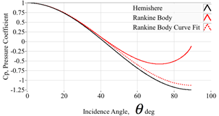
Figure 6 Comparing the surface pressure coefficient distributions for hemisphere and Rankine-body.

with the parameters {A, B} curve-fit to match the Rankine-Body curve at low incidence-angles, below 45o.

Note, that for lower-incidence angles, below 45^o, the Rankine and "Quasi-Newtonian" curves nearly coincide. However, at higher angles, the Rankine-Body curve diverges, with the minimum pressure occurring at approximately 70o incidence angle. Thus, for the purpose of a FADS system, if pressure ports are distributed on the windward surfaces at lower incidence angles -- below 45^o -- it is possible to accurately represent the surface pressure distributions for both the hemisphere and Rankine probe by a quasi-Newtonian model of Equation (16),

$\begin{array}{l} Hemisphere\to \left[\begin{array}{l}A=2.5\\ B=-1.25\end{array}\right]\\ C{p}_{\theta }=A.{\cos }^2\theta +B,\to \\ Rankine Body\to \left[\begin{array}{l}A=2.13284\\ B=-1.13284\end{array}\right]\end{array}$   (16)

In general, if the pressures are sensed in wind-ward facing direction near the stagnation region, the form of this model can be accurately "fit" to a wide variety of blunt-body shapes. Cobleigh, et al.,¹⁷ present calibration data for a range of blunt-shapes normally encountered on a range of flight vehicles. The form of this simple model is convenient for calculating the airdata state from a measured surface pressure distribution using the Triples algorithm.²¹ This approach allows a closed-form inverse solution to be calculated in near real time. The FADS Triples solution algorithm will be discussed in detail in the next section. It must be recognized that the theoretical solutions presented in the previous section were derived for simple, isolated bodies superimposed in the flow. For a real world-configuration the effects of the trailing afterbody or support mechanism must be accounted. For an aircraft this would include the upwash and compression induced by the wings and empennage. For a probe inserted in a wind tunnel, the afterbody effects would include effects of the mounting sting flow-compression, upwash, and associated tunnel blockage. These effects are compensated-for by fitting the coefficients {A, B} as a function of local angle-of-attack and tunnel airspeed. This "calibration" procedure will be discussed later in the "Results and Discussion" section of this paper.

FADS solution methodology

For this work, the surface pressure distributions are used to estimate the airdata reference state using the Triples algorithm as derived by Ref. ²² Although a wide range of solutions methods have been developed and applied, Refs.^19–21,27 the authors believe that the Triples approach offers the best combination of simplicity, reliability, and accuracy; and that approach will be used for this analysis. This section lays out the steps that are used for estimating the airdata state using the Triples algorithm,

Solving for the angle-of-attack

As illustrated Figure 7 for a Rankine-Body, the surface position of a particular pressure port can be described in terms of two polar coordinates, "cone" Θ and “clock" ϕ angles. The total surface incidence angle θ at non-zero angle-of-attack α and/or sideslip β can be calculated by taking the inner product of the local flow direction vector and the surface normal,

$\overrightarrow{V}.\overrightarrow{n}=\cos \theta =\left[\begin{array}{l}\cos \alpha \cos \beta \cos \theta +\\ \sin \beta \sin \Theta sin\varphi +\\ sin\alpha cos\beta sin\Theta cos\varphi \end{array}\right]$   (17)

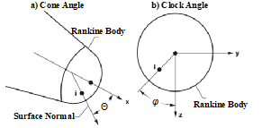
Figure 7 Local surface coordinate, cone and clock angle definitions.

where,

$\overline{V}=\left[\begin{array}{l}u\\ v\\ w\end{array}\right]=V_{\infty }.\left[\begin{array}{l}\cos \alpha \cos \beta \\ \sin \beta \\ sin\alpha cos\beta \end{array}\right] \overline{n}=\left[\begin{array}{l}\cos \Theta \\ \sin \Theta \sin \varphi \\ sin\Theta cos\varphi \end{array}\right]$   (18)

As shown Figure 8, consider three pressure ports on a "meridian" running through axis of symmetry. By taking differences of this "triple," using the quasi-Newtonian Model, the pressure differences can be written explicitly in terms of the total incidence angles at each location.

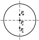
Figure 8 Pressure triples arrangement on vertical meridian.

$\frac{C_{p_{{}_u}}-C_{p_c}}{C_{p_{{}_c}}-C_{p_{{}_L}}}\equiv \frac{p{}_u-p_c}{p_c-p_L}\equiv \frac{{\Gamma }_{u,c}}{{\Gamma }_{c,L}}=\frac{{\cos }^2{\theta }_u-{\cos }^2{\theta }_c}{{\cos }^2{\theta }_c-{\cos }^2{\theta }_L}$   (19)

Along the central meridian sin () =0, and Eq. (19) can be written in terms of the flow direction angles as

$\begin{array}{l}\frac{{\Gamma }_{u,c}}{{\Gamma }_{c,L}}=\frac{{\left(\cos \alpha \cos {\Theta }_u-\sin \alpha \sin {\Theta }_u\cos {\varphi }_u\right)}^2{\cos }^2\beta -{\left(\cos \alpha \cos {\Theta }_c-\sin \alpha \sin {\Theta }_c\cos {\varphi }_c\right)}^2{\cos }^2\beta }{{\left(\cos \alpha \cos {\Theta }_c-\sin \alpha \sin {\Theta }_c\cos {\varphi }_c\right)}^2{\cos }^2\beta -{\left(\cos \alpha \cos {\Theta }_L-\sin \alpha \sin {\Theta }_L\cos {\varphi }_L\right)}^2{\cos }^2\beta }=\\ \frac{{\left(\cos \alpha \cos {\Theta }_u-\sin \alpha \sin {\Theta }_u\cos {\varphi }_u\right)}^2-{\left(\cos \alpha \cos {\Theta }_c-\sin \alpha \sin {\Theta }_c\cos {\varphi }_c\right)}^2}{{\left(\cos \alpha \cos {\Theta }_c-\sin \alpha \sin {\Theta }_c\cos {\varphi }_c\right)}^2-{\left(\cos \alpha \cos {\Theta }_L-\sin \alpha \sin {\Theta }_L\cos {\varphi }_L\right)}^2}\end{array}$   (20)

As derived by Whitmore, et al.,²¹ the solution of Eq. (20) can be written explicitly as

$\alpha =\frac{1}{2}{\tan }^{-1}\left(\frac{A}{B}\right)$   (21)

where,

$\begin{array}{l}A={\Gamma }_{u,L}{\sin }^2{\Theta }_c+{\Gamma }_{c,u}{\sin }^2{\Theta }_L+{\Gamma }_{L,c}{\sin }^2{\Theta }_u\\ B={\Gamma }_{u,L}\cos {\varphi }_c\sin {\Theta }_c\sin {\Theta }_c+{\Gamma }_{c,u}\cos {\varphi }_L\sin {\Theta }_L\sin {\Theta }_c+{\Gamma }_{L,c}\cos {\varphi }_u\sin {\Theta }_u\sin {\Theta }_u\end{array}$   (22)

A similar solution procedure using three ports along the lateral meridian, where, $\varphi ={90}^{o}or\varphi ={270}^o$ can be used to calculate the flank angle-of-attack ${\alpha }_F$ . Given α and α_F, the true angle-of-sideslip β is calculated using the geometric relationship,

$\beta ={\tan }^{-1}\left[\tan ({\alpha }_F).cos\alpha \right]$   (23)

Noise rejection

Using three pressure ports and the triples algorithm to estimate the angle-of-attack is equivalent to a higher order spline fit with the numerator sensing the flow direction, and the denominator scaling for the effects of dynamic pressure. The resulting calculation is rather sensitive to noise in the measured pressures. Providing additional sensing locations mitigates the noise sensitivity, increases redundancy options, and results in a system which gives overall superior performance. In general, for N pressure ports along the meridian, there exists

$N_{triples}=\frac{\left(N!⋰3!\right)}{\left(N-3\right)!}$   (24)

total possible combinations of pressure triples.³² Figure 9 depicts such a redundant system with 5-pressure ports distributed symmetrically along the vertical meridian. In this configuration there is a single center port, and two ports each distributed above and below the horizontal symmetry plane. Given a data set with 5 members, as depicted by Figure 9,

$\overline{P}=\{P_{L_1},P_{L_2},P_c,P_{u_1},P_{u_2}$ ,

there exists a total of 10 total possibilities for pressure triples combinations. The ports highlighted in red on Figure 9 show these 3-port combination possibilities.

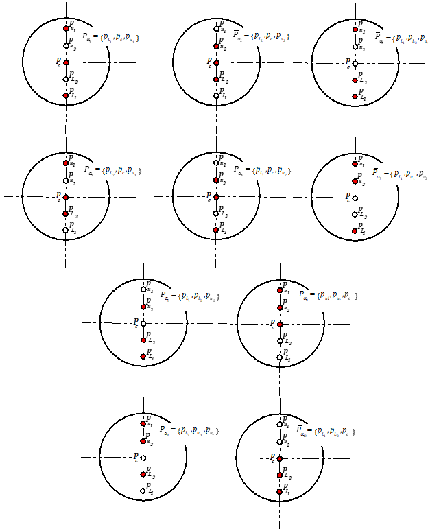
Figure 9 Possible angle-of-attack triples combinations.

Using the algorithm of Eqns. (17) - (21) to solve for angle of attack for each triple combination, gives 10 independent measures of the angle-of-attack. Taking a weighted averaging of these solutions, acts as a finite impulse filter,³³ providing a significant measure of noise rejection from the result. Similar procedures can be used to calculate the flank-angle-of attack and angle-of-sideslip.

Complete air data state solution

Given the mean effective angle-of-attack solution  , and assuming the pressure matrix layout of Figures 9, the vector of quasi-Newtonian pressure coefficient model estimates are calculated for each port location,

where

${\stackrel{⌢}{C}}_p=\left[\begin{array}{l}A.{\cos }^2{\theta }_{L_1}+B\\ A.{\cos }^2{\theta }_{L_2}+B\\ A.{\cos }^2{\theta }_c+B\\ A.{\cos }^2{\theta }_{u_{{}_1}}+B\\ A.{\cos }^2{\theta }_{u_{{}_2}}+B\end{array}\right] \overline{\theta }=\cos \beta .\left[\begin{array}{l}\cos \widehat{\alpha }\cos {\Theta }_{L_1}+\sin \widehat{\alpha }\sin {\Theta }_{L_1}\cos \varphi {}_{L_1}\\ \cos \widehat{\alpha }\cos {\Theta }_{L_2}+\sin \widehat{\alpha }\sin {\Theta }_{L_2}\cos \varphi {}_{L_2}\\ \cos \widehat{\alpha }\cos {\Theta }_c+\sin \widehat{\alpha }\sin {\Theta }_c\cos \varphi {}_c\\ \cos \widehat{\alpha }\cos {\Theta }_{u_{{}_1}}+\sin \widehat{\alpha }\sin {\Theta }_{u_1}\cos \varphi {}_{u_1}\\ \cos \widehat{\alpha }\cos {\Theta }_{u_2}+\sin \widehat{\alpha }\sin {\Theta }_{u_2}\cos \varphi {}_{u_2}\end{array}\right]$   (25)

and the sensed pressure buffer is related to the dynamic and static pressure by,

$\overline{P}=\left[\begin{array}{l}{P}_{L_1}\\ P_{L_2}\\ P_c\\ P_{u_1}\\ P_{u_2}\end{array}\right]=\left[\begin{array}{l}{\stackrel{⌢}{C}}_{p{L}_1}.q_c+p_{\infty }\\ {\stackrel{⌢}{C}}_{p{L}_2}.q_c+p_{\infty }\\ {\stackrel{⌢}{C}}_{p_c}.q_c+p_{\infty }\\ {\stackrel{⌢}{C}}_{p{u}_1}.q_c+p_{\infty }\\ {\stackrel{⌢}{C}}_{p{u}_2}.q_c+p_{\infty }\end{array}\right]$   (26)

Writing Eq. (26) in vector form,

$\overline{P}=\left[{\stackrel{⌢}{C}}_p|1\right].\left[\begin{array}{l}{q}_c\\ p_{\infty }\end{array}\right]$   (27)

the optimal least-squares solution can be calculated by using the pseudo-inverse method

$\left[\begin{array}{l}{q}_c\\ p_{\infty }\end{array}\right]={\left\{\left[\begin{array}{l}{\stackrel{⌢}{C}}_p\\ \dots \\ 1111\end{array}\right].\left[\begin{array}{l}{\stackrel{⌢}{C}}_p| 1\\ 1\\ 1\\ 1\\ 1\end{array}\right]\right\}}^{-1}\left[\begin{array}{l}{\stackrel{⌢}{C}}_p\\ \dots \\ 1111\end{array}\right].\overline{P}$   (28)

Using Cramer's rule,³⁴ the optimal solution for dynamic and static pressure can be written in closed form,

$\left[\begin{array}{l}{q}_c\\ p_{\infty }\end{array}\right]=\frac{\left(\begin{array}{cc}N& -{\displaystyle \sum _{i=1}^N{C}_{P_i}}\\ -{\displaystyle \sum _{i=1}^N{C}_{P_i}}& {\displaystyle \sum _{i=1}^N{(C_{P_i})}^2}\end{array}\right)\left(\begin{array}{l}{\displaystyle \sum _{i=1}^N{C}_{P_i}}.p_i\\ {\displaystyle \sum _{i=1}^N{p}_i}\end{array}\right)}{N.\left({\displaystyle \sum _{i=1}^N{(C_{P_i})}^2}\right)-\left({\displaystyle \sum _{i=1}^N{C}_{P_i}}\right)}$   (29)

In Eq. (29), N is the number of pressures in the data buffer, and in the case of Figure 9, N is equal to 5. Given the static and dynamic pressure, the airspeed, mach number, and other desired parameters are calculated from Bernoulli’s law, and standard airspeed relationships. Figure 9 presents a flow chart summarizing the FADS "Triples" solution algorithm.

A series of Monte Carlo simulation studies were performed in order to assess the measurement requirements for the proposed low speed wind tunnel tests. For this analysis the Rankine-Body flow model of Section IV.b is used to predict the local surface pressure distributions, aligned along the vertical meridian as in Figure 10, as a function of airspeed and angle-of-attack. The Rankine model accounts for a freestream angle-of-attack by allowing for small perturbations of the local flow incidence angle, where,

$\tan \theta =\frac{\tan \phi +(\pi -\phi ).(1+ta{n}^2\phi )}{ta{n}^2\phi }=\tan (\alpha -\Theta .\cos \varphi )$   (29)

Figure 10 Flow chart of FADS "triples" solution algorithm.

In Eq. (29) N is the assumed angle of attack,  is the port geometric incidence-angle of the port, and is the port clock angle. In this approximation the introduced angle-of-attack has the effect of increasing the total flow angle for ports that lie on "top" of the body above the horizontal axis of symmetry, and the effect of decreasing the total flow incidence-angle for ports that line in the "bottom" of the model below the horizontal axis of symmetry. Using this approximation, the Rankin polar angle  is numerically solved from Eq. (29) , and  the associated pressure coefficient and absolute surface pressure is calculated as a function of airspeed using Eq. (12), and assuming a sea level air density.

The surface pressure are corrupted assuming Gaussian-distributed white noise (GWN).³⁵ The noise contamination is partitioned as two pieces added together, 1) a bias value, and 2) a random value. For the bias noise, at the beginning of each Monte-Carlo run the noise is distributed as GWN among the ensemble of pressure ports, and remains fixed throughput the duration of the run. For the random noise component, the GWN is allowed to vary amongst the ensemble of ports and for each airspeed condition throughout the run. Using the generated pressures, the FADS solution algorithms of the previous section are used to re-calculate the angle-of-attack, airspeed, and dynamic pressure for each Monte-Carlo run. The differences are plotted as a scatter plot as a function of airspeed, and for each of 4 angle-of-attack groupings, {0^o, 5^o, 10^o, and 15^o }. Figures 11&12 show typical simulation results for two different angles-of-attack, 0o and 15o.

Presented on Figure 11 are the simulation results for 0o angle-of-attack. Plotted are angle-of-attack dynamic pressure, and airspeed error scatter-plots at 0o angle-of-attack, for the two assumed noise levels of the previously-described Fig. 1, i.e. +0.5 psf (0.024 kPa), and +0.1 psf (0.005 kPa). For this analysis the error is distributed as 33% bias, and 67% random. Note that the associated estimation error levels are a highly non-linear function of the introduced noise level, and the error levels assuming the higher-noise level are approximately and order of magnitude higher. Figure 12 presents similar comparisons for the 15o angle-of-attack simulations runs. Note that the random error levels do not substantially grow at the higher angles of attack. However, the systematic errors are significantly higher for the 15^o case, and these systematic errors levels increase with airspeed. The systematic errors are likely a result of the small perturbation model used to introduce angles-of-attack into the Rankine-Body pressure model, and demonstrates the limitations of the quasi-Newtonian model to account for these perturbations. Recall that for the 15o angle-of-attack condition, the upper 45o cone angle port has a total incidence angle of 60o. This upper flow incidence-angle is sufficiently large that the Newtonian model is no longer an accurate representation of the Rankine-Body. Based on these observations, it is likely that pressure measurement accuracies of at least of +0.10-0.20 lbf/ft² (0.005-0.01 kPa) will be required to accurately sense the airdata set over the entire UAV operating range. These requirements are very stringent, and at the margin of the pressure transducers measurement accuracies that are typically available for aviation-grade, Commercial Off-the-Shelf (COTS) equipment.

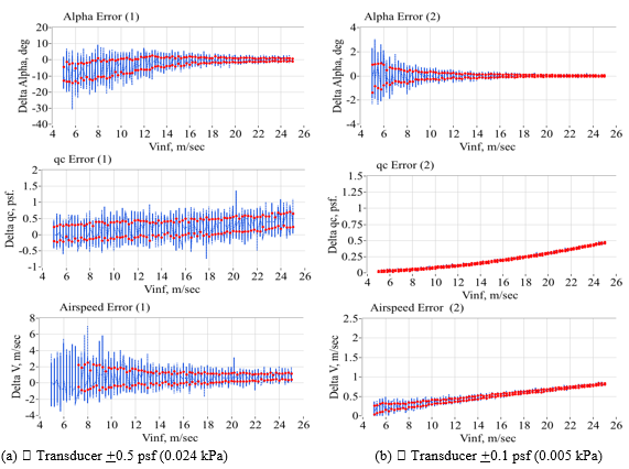
Figure 11 Monte Carlo scatter plot error summary for two different noise levels, at 0o angle-of-attack.

Figure 12 Monte Carlo scatter plot error summary for two different noise levels, at 15o angle-of-attack.

This section describes the instrumentation and test systems used to support the low speed wind tunnel tests. The probe design and manufacture will be described first, followed by the development and manufacture of the wind tunnel sting support systems. The probe pressure sensing systems and operating characteristics and will be described next. Finally, the wind tunnel systems, instrumentation, and operating characteristics will be described.

Airdata probe design

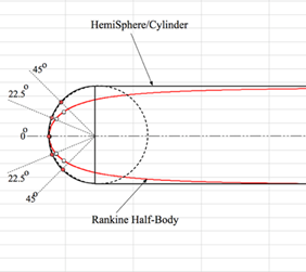
For the feasibility assessment, it was decided to test two similarly-sized probes, one with a hemispherical-cylinder shape, and one with a Rankin body shape. These probes had ports 5-ports at cone angles arranged only in the vertical meridian, thus, only the angle of attack, dynamic pressure, and the associated airspeeds could be sensed by these probes. This design was for operational simplicity. It was reasoned that if angle-of-attack can be reasonably and accurately sensed at low speeds, then sensing angle-of-sideslip would present the same issues and accuracy results. Figure 13 compares the probe geometries. Table 1 lists the port cone and clock angles for these probes.

Figure 13 Hemispherical-head, and Rankine-body shape comparisons with 5 ports arranged at identical.

Airdata probe manufacture

The test probes were additively manufactured from polycarbonate (Veroclear®) using a Polyjet (Objet 260 Connex3) 3D-printer. For both designs the probes were printed with "built-in" surface ports pressure transmission paths. Figure 14 shows these design layouts for the Rankine and hemispherical-head probes. Each probe had a major diameter of 1.25" (31.75 mm), and the 5 pressure-transmission paths used 0.5" (1.27 mm) surface ports, laid out at 22.5^o degree surface-normal spacing intervals. Barbed plastic tube fittings were bonded into probe outlet holes, and flexible tubing was used to transmit pressure to the sensing pressure transducer. 

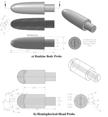
Figure 14 3-D printed probe layouts.

  The probe support sting and fairing were printed from Acrylonitrile Butadiene Styrene (ABS) at full density using a Fortus 250-MC, Fused-Deposition Manufacturing (FDM) printer.  The sting was mounted using a telescope sight and support rail. Probe angles-of-attack were set by mounting the support rod to a precision tilt table, originally designed for use on milling tables.  Figure 15 shows the hemispherical probe as mounted and centered in the wind tunnel test section. At the 15^o angle-of-attack set point, estimated frontal areas of the probe, sting fairing, and support mount are estimated to be approximately 130 cm². The wind tunnel test section cross section at the test area is approximately 3716 cm². Thus, the maximum wind tunnel blockage is approximately 3.5%. This value is considered to be acceptable for low-speed test conditions.

Figure 15 FADS probe mounted in wind tunnel test section.

Probe test instrumentation

The probe instrumentation consisted of two parts, 1) a 16-port pressure scanner, and 2) a tilt-angle sensor mounted to the sting-support tilt-table. Wind-tunnel operating conditions were sensed by a separat set of pressure instrumentation. Figure 16 presents a block diagram of the probe instrumentation system. Figure 17 shows the probe instrumentation test deck.

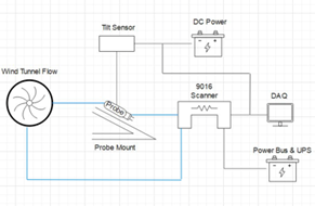
Figure 16 Probe instrumentation schematic.

Figure 17 Probe instrumentation test-deck.

Pressure scanner

The pressure sensing system used to measure the probe pressure data was selected based on the accuracy requirements as established using the Monte-Carlo simulation analysis, to be presented later in the Results and Discussion Section of this paper. The selected system is the Measurement Specialties® smart digital pressure scanner, Model 9016.  The system consists of an intelligent module with 16 integral pressure transducers and a pneumatic calibration manifold. The module output engineering unit pressure data, and is interfaced through a standard 10-Base-T Ethernet communications with TCP/IP protocol.

Each transducer is individually addressable. Each of the 9016 pressure transducer scale coefficients are stored onboard the unit processor in non-volatile memory. The digital output has 16-bit resolution. The sensing Wheatstone bridges feature a "differential" reading mode where the output pressure units result from the difference between the input pressure and the "backside" reference pressure. For this test series the reference pressure was tied into the wind-tunnel static pressure source, and the scanner output at each port represented the local dynamic pressure reading.  Figure 18 shows this arrangement. The Setra® pressure transducers depicted by Figure 18 are a part of the wind-tunnel instrumentation and control system, and will be described later in this section. Pre-test calibrations demonstrated that the transducer scale coefficients were highly stable and do not need recalibration during testing. Before each test run the transducer bridges were "zeroed" by taking a sample data set of up to 100 points for each transducer bridge with the wind tunnel inoperative. This sample was averaged for each of the individual transducers, stored in memory, and subtracted from the data readings for the subsequent tests. After re-zero, each transducer bridge has a manufacturer-guaranteed accuracy level of better than +0.15% of full-scale. The scanner used for this testing campaign has a full-scale differential pressure range of 20 in. H₂O (103.94 psf); thus, the expected accuracy for each pressure reading is better than +0.03 in. H₂O or approximately +0.156 psf, or slightly than the +0.1 psf error values assumed for Figures 1 (c)&(d).

Figure 18 9016 Intelligent pressure scanner module with reference port configuration.

Tilt angle sensor

The set-point for the model geometric angle-of-attack was sensed using a tilt-angle sensor mounted to the previously-described tilt-table. This sensor features dual-axis pitch and roll outputs, with a 0-5VDC output over a +60o operating range. When nulled for initial offset, the manufacturer's specification for absolute accuracy is approximately +0.1o. The analog output from the tilt sensor was digitized and recorded with a 16-bit miniature data-acquisition system.

Wind tunnel test systems

The USU recirculating wind tunnel,³⁶ designed and built by Engineering Laboratory Design in Lake City, MN,  features a 4 ft. long by 2 ft. wide by 2 ft. high test section. The 50 HP motor allows tunnel airspeeds of up to 50 msec. The recirculating tunnel slightly pressurizes and heats up during operating, and a water-cooled heat exchanges is used to maintain the tunnel stagnation temperature at a constant value.  The absolute static pressure level of the recirculating wind tunnel drops as the tunnel airspeed increases. Figure 19 shows this calibration correction, where the difference between the test section static pressure and the external ambient pressure is plotted as a function of the tunnel airspeed, and is fit with a linear least-squares curve. The tunnel airspeed is controlled using a Proportional/Integral/Derivative (PID) controller using the tunnel dynamic pressure as a feedback. The tunnel dynamic pressure is sensed via a pitot-static probe mounted at the test section inlet, with the differential pressure being sensed by the two Setra Pressure Systems transducers depicted in Figure 18. Here two pressure ranges are sensed, 1) a "low" pressure range of 0-3 In. H₂O (15.6 psf), and 2) a "high" pressure range of 0-15 In. H₂O (77.9 psf). Airspeed is calculated from dynamic pressure using ambient pressure and temperature sensed by a hand-held combined barometer/temperature sensing unit. Depending on the tunnel airspeed, either the "low" (V∞ < 30 m/sec) or "high" transducer is selected for the PID control. The manufacturer's specified accuracy for the Setra units is +1% of full scale or approximately +0.03 In. H₂O (0.16 psf), and +0.15 In. H₂O (0.78 psf). This level of sensing accuracy allows the PID controller to maintain the tunnel airspeed at an accuracy level of better than 0.25 m/s.

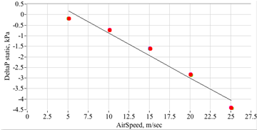
Figure 19 Wind tunnel static pressure correction to ambient.

This section reports on the wind tunnel test results. Table 2 summarizes the test matrix. For each configuration a total of 20 different test points were obtained. Each probe was tested at 5 different airspeeds varying from 5 to 25 m/s, and 4 different angles-of-attack varying from zero to 15o. Zero-airspeed baseline points were also measured. For each test The scanner data were collected by a stand-alone laptop running Lab VIEW as the logging software. The wind tunnel operation was controlled by a separate control computer.  The procedure was to first set the desired geometric angle-of-attack set point, then "zero" the pressure scanner transducer bridges at zero airspeed. As described in the previous section, the transducer zero task was accomplished by collecting a sample data set of up to 100 points for each transducer bridge, and averaging the results. The averaged values were stored in the test computer memory, and subtracted from the data readings for the subsequent test. The tunnel was subsequently started and allowed to stabilize at the commanded airspeed setting. Once the tunnel airspeed had stabilized, test data for both the FADS pressures and the tunnel conditions were logged. Ambient conditions were recorded in each file header. The FADS pressure data and tunnel conditions were time-synced and merged into a single file post-flight. Each data run was approximately 40 seconds in duration.

System calibrations

The effects of the mounting sting, tunnel blockage, and the probe afterbody were accounted for through a series of calibrations. Here, the wind tunnel reference conditions, airspeed, ambient pressure, and dynamic pressure, were used along with the pressure coefficient data to estimate the Newtonian flow model parameters {A, B} of Eq. (16). A systematic flow offset  was also estimated. This parameter accounts for asymmetric flow compression and upwash resulting due to the probe mounting sting. The algorithm used to estimate the calibration coefficients was an iterative, nonlinear-least squares algorithm.  Equation (31) shows the resulting calculation sequence. The algorithm starts with an initial guess for the flow parameters, typically the theoretical values from potential flow {A=2.25, B=-1.25}, and he subroutine iterates until convergence, updating the parameters after each iteration. Figure 19 presents these results. Fig. 19(a) plots the calibration data as derived for the Rankine Probe, and Fig. 19(b) plots the calibration data for the hemispherical-head probe. The Newtonian Model Coefficients {A,B}, and the flow correction parameter  plotted as a function of airspeed for the 4 different angle of attack ranges. The plotted data are a result of each data run, time-averaged over the duration of the run. Also note that the red constant lines in Figs. 19(a), and 19(b) that denote the theoretical fit coefficients, from Eqn. (16). Overall, both probes exhibit clean trends and curve fits. Both probes exhibit systematic effects, with the Rankine probe having a stronger effect due to angle-of-attack.

$\begin{array}{l}{\left[\begin{array}{l}A\\ B\\ \alpha \end{array}\right]}^{\left(j+1\right)}={\left[\begin{array}{l}A\\ B\\ \alpha \end{array}\right]}^{\left(j\right)}+{\left(\begin{array}{ccc}{\displaystyle \sum _i^{}{\cos }^4{\theta }_i{}^{(j)}}& {\displaystyle \sum _i^{}{\cos }^2{\theta }_i{}^{(j)}}& {\displaystyle \sum _i^{}{\cos }^2{\theta }_i{}^{(j)}.F_i{}^{(j)}}\\ {\displaystyle \sum _i^{}{\cos }^2{\theta }_i{}^{(j)}}& n& {\displaystyle \sum _i^{}{F}_i{}^{(j)}}\\ {\displaystyle \sum _i^{}{\cos }^2{\theta }_i{}^{(j)}.F_i{}^{(j)}}& {\displaystyle \sum _i^{}{F}_i{}^{(j)}}& {\displaystyle \sum _i^{}{F}_i{}^{2(j)}}\end{array}\right)}^{-1}\\ .\left[\begin{array}{l}{\displaystyle \sum _i^{}{\cos }^2{\theta }_i{}^{(j)}}.(C_{pi}-C_{pi}{}^{(j)}\\ {\displaystyle \sum _i^{}(C_{pi}-C_{pi}{}^{(j)})}\\ {\displaystyle \sum _i^{}{F}_i{}^{(j)}}.(C_{pi}-C_{pi}{}^{(j)})\end{array}\right]\end{array}$   (30)

where,

$\begin{array}{l}\cos {\theta }_i{}^{(j)}=\left(\cos {\alpha }^{(j)}\cos {\varphi }_i+\sin {\alpha }^{(j)}\sin {\varphi }_i\cos {\lambda }_i\right)\\ C_{pi}{}^{(j)}=A^{(j)}.{\cos }^2{\theta }_i{}^{(j)}+B^{(j)}\\ F_i{}^{(j)}\equiv \sin (2{\theta }_i{}^{(j)}).(cos{\alpha }^{(j)}\sin {\varphi }_i\cos {\lambda }_i-\sin {\alpha }^{(j)}\cos {\varphi }_i)\end{array}$

Overall, both probes exhibit clean, monotonic data trends. The data of Figure 20 were curve-fit using a linear model, where $V_{\infty }$ is the first independent variable, and effective $\alpha$ is the second independent variable. Table 3 lists the coefficients for the calibration table.

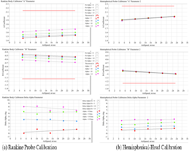
Figure 20 Calibration plots for the Rankine and hemispherical-head probes.

Calibrated pressure coefficient distributions

Figure 21 shows a typical pressure distribution data plot, collected at 5 m/s and 25 m/s airspeed and 0^o and 5^o angle-of-attack set points. These pressure coefficient Cp data, plotted as a function of the port true incidence angle, are compared against the theoretical models for each probe. For the Cp calculation, the dynamic pressure was taken from the Setra low-pressure (high resolution) reading, and the static pressure was calculated from the logged barometric pressure, corrected for airspeed using the curve-fit of Figure 19. For all plotted Cp data points the incidence angle is corrected to account for the systematic angle of attack-errors from Figure 20. The plotted red and blue data points are the sensed Cp results for the Rankine-Body and Hemispherical head probes. The plotted curves include the theoretical curves for the Hemisphere and Rankine-Body from Eqs. (5) and (12), and the best-fit curves for the quasi-Newtonian model, from the calibration plots of Figure 20. Note that the measured results for both probes exhibit higher Cp values, indicating significant flow compression due to the mounting apparatus and probe afterbody, and possibly some amount of tunnel blocking. But for each plot the Cp data points exhibit consistent monotonic behavior, showing that the effects of noise are minimal for the calibration fits.

FADS error assessments and comparisons

Using the sensed scanner pressure data, together with the curve-fit calibrations of Table 3, the FADS solution method depicted by the flow chart of Figure 10, were applied to calculate the "point-by-point" time-history estimates of the airdata values. The first step in this process is calculation of the angles-of-attack for each of the pressure-triples as shown by Figure 9. Recall from Eq. (21) that the triples solution does not require knowledge of the Newtonian flow model parameters {A, B}, and the solution returns an aerodynamic or "effective" angle of attack ${\alpha }_e$ . 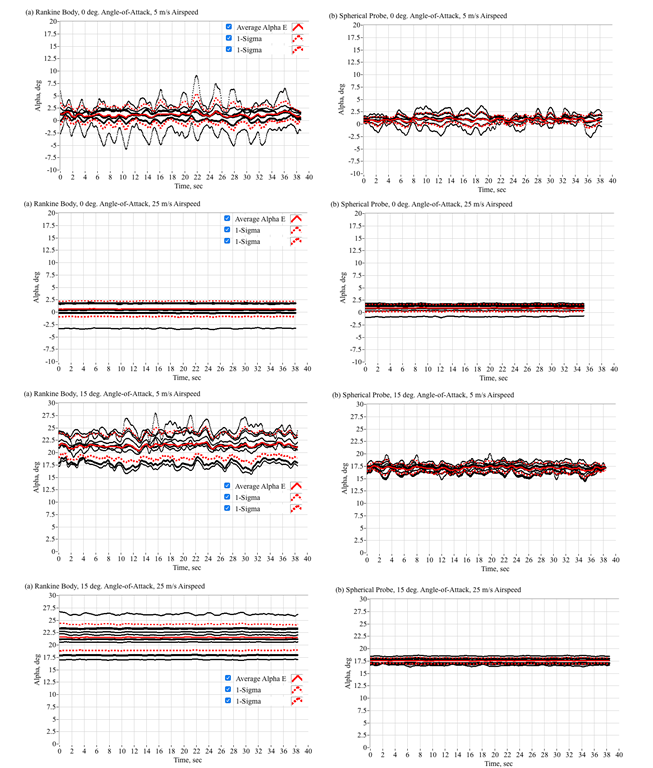Figure 22 compares the individual solutions for the ${\alpha }_e$ for the Rankine and spherical probes for the example data of Figure 21, at 0o and 15o reference angle-of-attack, and 5 and 15 m/s reference airspeed. Plotted are the individual ${\alpha }_e$ solutions time histories for each triple, as well as the ensemble means and standard deviations from amongst the set of triples solutions. Note that the hemispherical-head probe exhibits significantly less systematic dispersions amongst the individual solutions, when compared to the Rankine-Body probe solutions. This observation clearly shows that the quasi-Newtonian model is a better fit for the hemispherical shape than it is for the Rankine shape.

Figure 21 Comparing the pressure distributions for Rankine-body and hemispherical-head probes, {0o, 15o} angles-of-attack, and {5, 25 m/s} airspeeds.

Figure 22 Comparing the individual and mean the triples solutions for the Rankine-body and hemispherical head shapes.

Once the Mean value for the effective angle of attack-is-calculated, the starting values {A, B} are taken from Eq. (16), and Eqs. (25) and (29) are used to calculate qc and p∞, and V_∞ airspeed is re-calculated based on the mean ambient air density (from the measured barometric conditions). Using the calculation for V_∞ the coefficients {A, B} are re-evaluated, and the process is iterated to convergence, typically 2 or 3 iterations, for each time frame. Once the calculation is converged, the final airspeed is used to evaluate the δα correction, allowing the "true" geometric angle-of-attack to be calculated.  Figure 23 shows a typical result where the sensed tunnel airspeed, angle of attack, and dynamic pressure are compared against the reconstructed FADS estimates for the Hemispherical probe data, with the tunnel airspeed set at approximately 25 m/sec, and the geometric angle-of-attack of the probe at 150 nominal set point. The Root-Mean-Square (RMS) and mean-error/residual for each parameter is also displayed. Note that the FADS reconstruction, calculated using only the scanner (probe) pressure data, agrees well with the independently calculated tunnel reference conditions. Figure 24 summarizes the RMS error/residual results for both probes, calculated across the range of test airspeed and angle-of-attack conditions of Table 2.

Figure 23 Comparing the reconstructed fads air data estimates against the wind-tunnel reference conditions, hemispherical-head probe.

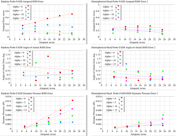
Figure 24 FADS estimate error summary for Rankine and hemispherical-head probe analyses.

For both probes the FADS airspeed estimate is accurate to better than 0.75 m/sec over the entire airspeed range. The angle-of-attack errors are less than 1 degree, and it is reasonable to assume that this value is within the uncertainty to which the probe is aligned geometrically within the tunnel. Both probes reconstruct the tunnel dynamic pressure very accurately, with maximum errors/residuals of less than 0.012 kPa (0.00174 psi) and 0.005kPa (0.00073 psi) for the Rankine and Hemispherical Probes, respectively.

The Rankine probe reconstruction exhibits a larger total systematic error than does the hemispherical probe. As shown by Figures 20(c)&(d), at the highest test angles-of-attack, 15o geometricor α 22.97^o ${\alpha }_e$ , the upper ports on the Rankine body lie at incidence angles that are higher than 45o, where the quasi-Newtonian model is known to not be a good fit. Thus, the observed systematic errors are very likely indicative of the Newtonian model having insufficient degrees of freedom entirely capture the flow properties. This result confirms the previous discussion of Figure 6. For the Rankine-Body probe.

Proposed future work

Clearly, for applications to more highly-elliptical leading edges or forebody shapes, adapting a higher-order flow model is desirable. If the quasi-Newtonian model is extended slightly, to allow for an incidence angle scaling parameter, ε

$C_{p_{{}_{\theta }}}=\left(A.{\cos }^2\epsilon .\theta +B0\right)$   (31)

then, the range of curve-fit applicability for the Rankine-body is extended to significantly higher incidence angles. Figure 25 shows this model extension, where {A=1.6164, B=-0.6164, and ε= 1.19172}.  Here the region of fit accuracy is extended up to beyond 70 degrees. It must be noted that when this model extension is applied, the triples algorithm no-longer allows a closed-form solution. Instead the solution for each triple must be iteratively determined,

${\stackrel{⌢}{a}}^{(n+1\text{})}={\stackrel{⌢}{a}}^{(n)}+\frac{\left({\Gamma }_i{}_{jk}\right).\cos (2.\epsilon .{\theta }_j)-{\Gamma }_i{}_{jk}\cos (2.\epsilon .{\theta }_k)-\cos (2.\epsilon .{\theta }_i)}{2.\epsilon \left[\left({\Gamma }_i{}_{jk}+1\right).\sin (2.\epsilon .{\theta }_j).\cos {\varphi }_i--{\Gamma }_i{}_{jk}\sin (2.\epsilon .{\theta }_k).\cos {\varphi }_k-\sin (2.\epsilon .{\theta }_i).\cos {\varphi }_i\right]}$   (32)

Figure 25 Extending the Quasi-Newtonian model to better fit Rankine-body shape.

In Eq. (32) n is the iteration index, and

${\Gamma }_i{}_{jk}=\frac{{\cos }^2\epsilon .{\theta }_i-{\cos }^2\epsilon .{\theta }_j}{{\cos }^2\epsilon .{\theta }_j-{\cos }^2\epsilon .{\theta }_k}=\frac{\cos (2.\epsilon .{\theta }_i)-\cos (2.\epsilon .{\theta }_j)}{\cos (2.\epsilon .{\theta }_j)-\cos (2.\epsilon .{\theta }_k)}$   (33)

Preliminary investigations have determined that the method of Eqs. (31) - (33) significantly reduce the associated systematic errors for the Rankine-body data, and is quite useful for post-test analysis. However, it also occurs that the current iteration methods are somewhat unstable, and can diverge in the present of measurement noise or other disturbances. This issue was previously experienced by Whitmore and Moes¹⁴ and may present operational issues for real-time inflight calculations. For the current state-of-the art, the authors hold that that the "Triples" approach of Figure 10 still presents the best combination of simplicity, sensing accuracy and system reliability.

Finally, the test results demonstrate that, using COTS pressure sensing technology, the FADS methods can calculate the entire airdata state at very low airspeed, with at least moderate accuracy levels. For higher sensing accuracy levels, it is likely that custom-developed, high accuracy, high-resolution pressure sensors will be necessary. One such option leverages sensing capabilities that have been developed for the medical and biological fields for applications such as ventilators, spirometers, CPAP, sleep diagnostic equipment, nebulizers, oxygen concentrators, and endoscopy. 
For medical applications, such systems have delivered up to 0.5% accuracy for differential pressure levels as low as +0.1 in H₂O (0.5 lbf/ft²).³⁷ Stability and accuracy of these systems under UAV flight conditions must be verified and documented.

The research objectives of this study investigates the feasibility of using Flush Air Data Sensing (FADS) System technology for air data measurements at the very low-airspeeds, where many Unmanned Aerial Vehicles (UAVs) operate. FADS is a non-intrusive alternative to pitot probes, where the vehicle nosecone, wing leading edge, or other aerodynamic surface can be configured with multiple pressure-ports distributed along the windward surface. Although FADS technology has been used for a variety of high-speed aircraft, FADS has never been applied to very low-airspeed flight regimes. Preliminary results from Monte Carlo simulation studies demonstrate that the measurement constraints at these low airspeeds are very stringent, with required accuracy levels between +0.10-0.20 lbf/ft2 (0.005-0.01 kPa) in order to accurately sense the airdata set over the low-speed UAV operating range from 5-25 m/s airspeed. These requirements are at the margin of pressure measurement accuracies typically from available aviation-grade, Commercial Off-the-Shelf (COTS) equipment.

In order to assess whether FADS technology can reliably measure airdata at very low airspeeds, this study reports on very low-speed wind tunnel tests of two 3-D printed forebody shapes: 1) a cylindrical body with a hemispherical head, and 2) a Rankine-body. These body shapes approximate a wide range of three-dimensional shapes, and act as a vehicle analog, accounting for both blunt leading edge and trailing afterbody flow characteristics. For this study the "probes" were printed with 5 pressure ports and the associated flow channels aligned at 0^o, +22.5^o and +45^o direction-angles along the vertical centerlines of the models. Probe surface pressures were sensed with a high resolution, but COTS-origin, pressure scanner. Sensed pressure data were curve-fit, developing quasi-potential flow calibration models for each probe, with coefficients compiled as a function of geometric angle-of-attack and tunnel airspeed. The calibration models account for end-to-end systematic effects, including the mounting sting flow compression, upwash, and tunnel blockage.

Using the derived calibration models and the sensed pressure data, the effective angles-of-attack were re-calculated using the well-known Triples algorithm. The associated airspeed and dynamic pressure are estimated from the sensed pressure data using non-linear regression. The resulting estimates are compared to the tunnel reference conditions. Generally, both probe shapes performed well, with the redundant 5-port arrangement allowing for significant noise rejection. At the highest test angles-of-attack, the upper ports on the Rankine-body lie at incidence angles that are higher than 45o, where the quasi-Newtonian model is known to not be a good fit. Thus, the observed higher systematic errors are very likely indicative of the Newtonian model having insufficient degrees of freedom entirely capture the flow properties. Clearly, for applications to more highly-elliptical leading edge or forebody shapes, adapting a higher-order flow model is desirable. A simple scaling factor on incidence angle may allow that extension.

The test results demonstrate that, using COTS pressure sensing technology, the FADS methods can calculate the entire airdata state at very low airspeed, with at least moderate accuracy levels. For higher sensing accuracy levels, it is likely that custom-developed, high accuracy, high-resolution pressure sensors will be necessary. Using FADS sensors for UAV airspeed measurements opens up a wide range possibility for flight control improvements.  Such improvements can significantly enhance reliability and flight safety. This outcome may allow increased use of UAVs for deliveries, search and rescues, surveillances, and other commercial industries that, due to reliability or safety concerns, have not yet adopted the use of UAV.

None.

The author declares that there is no conflict of interest.

1. What are the Main Applications of Drones. J Unmanned Aircraft. 2022.
2. Sankaralingham L, Ramprasadh C. A comprehensive survey on the methods of angle of attack measurement and estimation in UAVs. Chinese J of Aeronautics. 2020;33(3):749–770.
3. Haering EA. Airdata Measurement and Calibration. NADS TM-104316. 1995.
4. Gracey W. Summary of Methods of Measuring Angle of Attack on Aircraft. NACA TN 4351. National Advisory Committee on Aeronautics; Washington, DC; 1958.
5. Ellsworth JC, Whitmore SA. Simulation of a Flush Air-Data System for Transatmospheric Vehicles. J Spacecraft & Rockets. 2008;45(4).
6. Cary JP, Keener ER. Flight Evaluation of the X-15 Ball-Nose Flow-Direction Sensor as an Air-Data System. NASA TN D-2923. 1965.
7. Wolowicz CH, Gossett TD. Operational and Performance Characteristics of the X-15 Spherical, Hypersonic Flow Direction Sensor. NASA TN D-3070. 1965.
8. Siemers P, Wolf H, Flanagan P. Shuttle Entry Air Data System concepts applied to Space Shuttle Orbiter flight pressure data to determine air data - STS 1-4. AIAA 21st Aerospace Sciences Meeting; Reno, NV, USA; 1983.
9. Larson TJ, Siemers PJ. Subsonic Tests of an All-Flush-Pressure-Orifice Air Data System. NASA TP 1871. 1981.
10. Henry MW, Wolf H, Siemers Paul M. An Evaluation of Shuttle Entry Air Data System (SEADS) Flight Pressures - Comparisons with Wind Tunnel and Theoretical Predictions. AIAA Paper # 88-2052, 1988, 15th AIAA Aerodynamic Testing Conference; San Diego, CA; 1988.
11. Larson TJ, Whitmore SA, Ehernberger LJ, et al. Qualitative Evaluation of a Flush Air Data System at Transonic Speeds and High Angles of Attack. NASA TP 2716. 1987.
12. Whitmore SA, Moes T, Larson TJ. Preliminary Results from A Subsonic High Angle-of-Attack Flush Air Data Sensing (HI-FADS) System: Design, Calibration, And Flight Test Evaluation. NASA TM-101716. 25th AIAA Aerospace Sciences Conference; Reno, NV; 1990.
13. Whitmore SA, Moes TR. The Effects of Pressure Sensor Acoustics on Airdata Derived from a High-Angle-of-Attack Flush Airdata Sensing (HI_FADS) System. NASA TM-101736. 26th AIAA Aerospace Sciences Conference; Reno, NV; 1991.
14. Whitmore SA, Moes TR. Failure Detection and Fault Management Techniques for a Pneumatic HI-FADS System. NASA TM-4335. 27th AIAA Aerospace Sciences Conference; Reno, NV; 1992.
15. Whitmore SA, Moes TR, Czerniejewski MW, et al. Application of a Flush Airdata Sensing System to a Wing Leading Edge (LE_FADS). NASA TM 104267. 28th AIAA Aerospace Sciences Conference; Reno, NV; 1993.
16. Whitmore SA, Moes TR. Measurement Uncertainty and Feasibility Study of a Flush Airdata System for a Hypersonic Flight Experiment. NASA TM 4627. 1994.
17. Whitmore SA, Davis RJ, Fife JM. In-Flight Demonstration of a Real-Time Flush Airdata Sensing (RT_FADS) System. NASA TM 104314. 30th AIAA Aerospace Sciences Conference; Reno, NV; 1995.
18. Cobleigh BR, Whitmore SA, Haering EA Jr, et al. Flush Airdata Sensing (FADS) System Calibration Procedures and Results for Blunt Forebodies. NASA TP-209012. International Space Planes and Hypersonic Systems and Technologies; Norfolk, VA, United States; 1999.
19. Crowther WJ, Lamount PJ, Laurence DRP. Neural Network Approach to the Calibration of a Flush Air Data System. Aeronautical Journal. 2001;105(1044):85–95.
20. Rohloff TJ, Whitmore SA, Catton I. Air Data Sensing from Surface Pressure Measurements Using a Neural Network Method. AIAA Journal. 1998;36(11):2094–2101.
21. Rohloff TJ, Whitmore SA, Catton I. Fault-Tolerant Neural Network Algorithm for Flush Air Data Sensing. J Aircraft. 1999;36(3):541–549.
22. Whitmore Stephen A, Cobleigh Brent R, Haering Edward A. Design and Calibration of the X-33 Flush Airdata Sensing (FADS) System. NASA TM-1998-206540. Research Engineering, NASA Dryden Flight Research Center; 30th AIAA Aerospace Sciences Conference; Reno, NV; 1995.
23. NASA Shuts Down X-33, X-34 Programs. Space.com.
24. Anon. NASA Armstrong Fact Sheet: X-38 Prototype Crew Return Vehicle. 2014.
25. Davis MC, Pahle JW, White JT, et al. Development of a Flush Airdata Sensing System on a Sharp-Nosed Vehicle for Flight at Mach 3 to 8. NASA TM-209017. 2000.
26. Gebhart C. Dream Chaser through Critical Landing Test, Prepares for Orbital Flights.
27. Laurence RL, Argrow BM. Development and Flight Test Results of a Small UAS Distributed Flush Airdata System. J of Atmos and Ocean Tech. 2018;33(5):1127–1140.
28. Anon. Rankine Oval, Aerodynamics for Students. Aerospace, Mechanical & Mechatronic Eng., Univ. of Sydney; 2005.
29. Kuethe AM, Chow CY. Foundations of Aerodynamics: Bases of Design. 4th ed. John Wiley & Sons; New York, USA; 1987. p. 86–93.
30. Anon. Rankine Oval, Aerodynamics for Students. Aerospace, Mechanical & Mechatronic Eng., University of Sydney; 2005.
31. Anderson JD, Modern Compressible Flow. 4th Ed, New York: The McGraw Hill Companies, Inc; 2021.
32. Glen S. Permutation, Combination and Derangement: Formula, Examples From Statistics HowTo.com: Elementary Statistics for the rest of us!
33. Rabiner LR, Gold B. Theory and Application of Digital Signal Processing. Prentice-Hall, Inc; Englewood Cliffs, New Jersey; 1975. p. 215–256.
34. Rade L, Westergren B. Beta Mathematics Handbook: Concepts, Theorems, Methods, Algorithms, Formulas, Graphs, and Tables. CRC Press; Boca Raton, FL, USA; 1990.
35. Anon. Gaussian White Noise, Appendix II. The Wiley Online Library.
36. Jensen M. What's New: Recirculating Wind Tunnel. Utah State Engineer; 2018.
37. Anon. NovaSensor P2705, Miniature Low Pressure Sensor Die. Amphenol Advanced Sensors.