Submit manuscript...
eISSN: 2576-4500

Aeronautics and Aerospace Open Access Journal

Research Article Volume 8 Issue 3

Blade shape optimization in hover and forward flight

Filipe Szolnoky Cunha,2 Tomás Ortiz1

1DEM, Instituto Superior Técnico, Universidade de Lisboa, Portugal
2IDMEC, LAETA, DEM, Instituto Superior Técnico, Universidade de Lisboa, Portugal

Correspondence: Filipe Szolnoky Cunha, Instituto Superior Técnico, Av. Rovisco País Nº1,1049-001 Lisboa, Portugal

Received: July 12, 2024 | Published: July 24, 2024

Citation: Ortiz T, Cunha FS. Blade shape optimization in hover and forward flight. Aeron Aero Open Access J. 2024;8(3):134-150. DOI: 10.15406/aaoaj.2024.08.00201

Download PDF

Abstract

Novel aircraft configuration, such as drones, have emerged during the last decades. This project aims to offer insights into drone development, enhancing its efficiency by means of rotor optimization utilizing well-established theoretical models based on blade element momentum theory for estimating thrust generation and power requirements at hover and forward flight. The impact on performance of chord and airfoils pitch angle, particularly focusing on the twist, which is how pitch changes along the blade, is analyzed, followed by optimizations of multiple chord and twist distributions at different flight conditions. Additionally, Computational fluid dynamics tools are employed to simulate resulting rotor geometries and to the baseline. Simulations and model predict power reductions of 3% to 17%, with negative twist rates and increased platform as main characteristics of most efficient geometries.

Keywords: drone, rotor, twist, chord, optimization, CFD

Abbreviations

AoA, angle of attack; BET, blade element theory; BEMT, blade element momentum theory; CFD, computational fluid dynamics; LSB, large separation bubbles; MRF, multiple reference frame

Introduction

In recent decades, the aviation industry has witnessed remarkable advancements, particularly with the emergence of drones, these new vehicles have rapidly gained prominence due to their versatility. As the demand for drone technology continues to grow, there is an inherent need to overcome technological challenges and drive innovation. The goal of this project is to provide new insights and analyze possible paths of evolution of small rotors, which can contribute to reduce power consumption and enhance performance capabilities such as range or autonomy. Large scale rotors, used in helicopters, have larger efficiencies than small scale rotors as pointed out by R. Cagnato,1 these inefficiencies are mainly related with the size of the rotors and its implication in their Reynolds flight regime (Low Reynolds,Re< 5.10 5 ) MathType@MTEF@5@5@+= feaagKart1ev2aaatCvAUfeBSjuyZL2yd9gzLbvyNv2CaerbuLwBLn hiov2DGi1BTfMBaeXatLxBI9gBaerbd9wDYLwzYbItLDharqqtubsr 4rNCHbGeaGqiVu0Je9sqqrpepC0xbbL8F4rqqrFfpeea0xe9Lq=Jc9 vqaqpepm0xbba9pwe9Q8fs0=yqaqpepae9pg0FirpepeKkFr0xfr=x fr=xb9adbaqaaeGaciGaaiaabeqaamaabaabaaGcbaqcLbsaqaaaaa aaaaWdbiaacIcacaWGmbGaam4BaiaadEhacaGGGcGaamOuaiaadwga caWG5bGaamOBaiaad+gacaWGSbGaamizaiaadohacaGGSaGaamOuai aadwgacqGH8aapcaaI1aGaaiOlaiaaigdacaaIWaWcpaWaaWbaaeqa baqcLbmapeGaaGynaaaajugibiaacMcaaaa@4C7E@ ,2 which implies bad aerodynamic efficiency. Consequently, it is important to analyze all the parameters related to rotor performance and try to enhance it. Among all the geometrical parameters defining rotor’s geometry, this project focuses on two: twist distribution and platform shape by means of chord distribution.

Improving the efficiency through geometrical optimization has historically been a matter of significant interest. There are multiple studies analyzing all the implications of geometry modification in rotor’s efficiency for large scale rotors. In fact, there are even theoretical optimal configurations with hyperbolic chord and twist distributions for hovering, as noted by Joanne L. Walsh,3 who also showed the benefits of tapered blades and negative twist not only for hovering but also for forward flight regime. However, the number of studies about small scale rotors is not that large. Moreover, the operation at low Reynolds has significant implications in the performance, which may affect to the final optimal geometries implying that general ideas of large scall rotors do not apply to small rotors. At low Reynolds, where viscous effects are dominant, it occurs complex phenomena that leads to low aerodynamic efficiency. Separation of the flow followed by reattachment leading to the formation of large separation bubbles, which are linked to poor lift/drag ratio. Those problems were pointed out by F. Bohorquez,4 who analyzed the effect of several geometrical parameters for rotors operating at (Re 6.10 4 ) MathType@MTEF@5@5@+= feaagKart1ev2aaatCvAUfeBSjuyZL2yd9gzLbvyNv2CaerbuLwBLn hiov2DGi1BTfMBaeXatLxBI9gBaerbd9wDYLwzYbItLDharqqtubsr 4rNCHbGeaGqiVu0Je9sqqrpepC0xbbL8F4rqqrFfpeea0xe9Lq=Jc9 vqaqpepm0xbba9pwe9Q8fs0=yqaqpepae9pg0FirpepeKkFr0xfr=x fr=xb9adbaqaaeGaciGaaiaabeqaamaabaabaaGcbaqcLbsaqaaaaa aaaaWdbiaacIcacaWGsbGaamyzaiablYJi6iaaiAdacaGGUaGaaGym aiaaicdajuaGpaWaaWbaaeqaleaajugWa8qacaaI0aaaaKqzGeGaai ykaaaa@4124@ . Bohorquez provides interesting conclusions about chord and twist, by performing test and creating hybrid models between theoretical approaches and computational fluid dynamics (CFD). He pointed out the benefits obtained by larger chords platforms opposite to optimal large-scale rotors, for which low chord produces low solidity being it beneficial. Bigger chords enhance aerodynamic efficiency, it implies larger Reynolds regime and lower thickness ratio of airfoils, which enhances performance at low Reynolds. Moreover, he remarked improvements due to negative twist and benefits of taper near the tip of the blade. Additionally, other researchers such as J. Winslow et al.,5 studied the performance of these rotors. Among its conclusions, they remark the differences with large scale rotors due to a bigger impact of profile loses, which diminishes the effectiveness of twist and chord modifications that aimed to reduce inflow loses by creating a more uniform distribution. Despite the improvement was not as large as it can be for larger scale rotors, they concluded that negative twist is necessary for enhancing aerodynamic performance. Moreover, like Bohorquez, They conclude that larger chords enhanced the performance and taper blades showed negligible benefits except for large reductions near the tips. Other scholars like J. Wiebe6 performed optimizations using theoretical models, characterizing the airfoils properties with simpler tools such as XFOIL software. He remarked the limitations of theoretical models. Moreover, he approached the optimization using MATLAB toolbox and implementing interesting distributions defined by spline curves for both chord and twist. However, the performance of small-scale rotos is not only carried out by theoretical models but in fact, for a proper comprehension more complex tools are required like: CFD or even experimental test. Kodchaniphaphong et al.,8 carried out CFD simulations that were compared against experimental test of small-scale rotors in both regimes: hovering and forward flight, showing good predictions. R. Cagnato and C. Vasconcelos,1,7 also used CFD for characterizing and analyzing more complex phenomena of the rotor’s performance, using different approaches for the same type of simulations, Multiple reference frame (MRF) and Sliding mesh.

Supported by the ideas of the current state of the art, this project pursuits the estimation of rotor performance and possible chord and twist distributions for improving it in hover and forward flight using MATLAB version R2022b,9 blade element momentum theory (BEMT) and airfoils properties estimated by software for preliminary designs tasks like XFOIL 6.99.10 Concluding with CFD simulations with Fluent by Ansys version 2021 R2.11

Theoretical concepts, MATLAB models and optimization

Next section contains the theoretical background required for the models as well as the assumptions and hypothesis assumed.

Low Reynolds regime and aerodynamic properties

As emphasized, the rotors of drones operate in a different Reynolds regime compared to large-scale rotors. This has implications for the model, not only because the aerodynamic efficiency is severely affected, as noted in,4 but also because it affects the typical assumptions made in blade theory.

At high Reynolds regimes, lift (Cl) and drag coefficients (Cd) barely depend on Reynolds number. Moreover, the behaviour with the angle of attack (AoA) is approximately linear for lift and quadratic for drag. However, due to the greater impact of viscosity and the presence of phenomena such as large separation bubbles (LSB), these assumptions cannot be kept at low Reynolds. Multiple studies have analyzed this regime and the performance of airfoils under these conditions,12 trying to understand the behaviour of airfoils.

It is crucial to estimate the aerodynamic properties of the airfoils (NACA 0012) (lift and drag coefficients, Cl, Cd) for the rotor models. As stated in14 XFOIL is an interesting tool due to its simplicity, time cost and fairly good results. Figure 1 shows a comparative against experimental data.
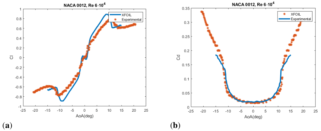
Figure 1 Comparison between XFOIL NACA 0012 data and experimental data from13 for Re=6 10 4 MathType@MTEF@5@5@+= feaagKart1ev2aqatCvAUfeBSjuyZL2yd9gzLbvyNv2CaerbuLwBLn hiov2DGi1BTfMBaeXatLxBI9gBaerbd9wDYLwzYbItLDharqqtubsr 4rNCHbGeaGqk0dg9crFfpeea0xh9v8qiW7rqqrFfpeea0xe9Lq=Jc9 vqaqpepm0xbba9pwe9Q8fs0=yqaqpepae9pg0FirpepeKkFr0xfr=x fr=xb9adbaqaaeGaciGaaiaabeqaamaabaabaaGcbaaeaaaaaaaaa8 qacaWGsbGaamyzaiabg2da9iaaiAdacqGHflY1caaIXaGaaGima8aa daahaaWcbeqaa8qacaaI0aaaaaaa@4082@
(a) Lift coefficient (Cl) versus angle of attack (AoA) (b) Drag coefficient (Cd) versus AoA.

XFOIL, which uses theoretical transition approach, is useful for low Reynolds computations as demonstrated by its developer M. Drela in.15 In terms of error, as pointed out in,6 it is optimistic predicting lift coefficient and stall point. Bohorquez3 discouraged using traditional thick airfoils for small rotors. However, blade airfoil section effect is not the goal of the project. NACA 0012 was chosen because it is one of the most studied airfoils, the amount of data available at low Reynolds was bigger and if required, fabrication would be easier due to its symmetry.

Theoretical background

Rotors performance models are based on Blade Element Momentum Theory (BEMT) adapted at each flight regime. This theory is a combination of two others: Momentum theory and Blade Element Theory (BET).

Momentum theory

Momentum theory assumes that a stream-tube, Figure 2, appears in the rotor vicinity. This 1-D theory uses conservation laws of: mass, momentum, and energy in the control volumes, above and below the rotor disk. All the hypothesis required for this theory are found in the book written by Leishmann.16
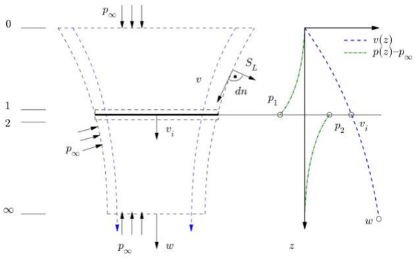
Figure 2 Scheme of the stream-tube with control volume definitions and lateral pressure distribution for Von Misses hypothesis.

After performing the mass, momentum and energy balances, it is obtained the next relationships with relate the thrust (T), induced power ( P i ) MathType@MTEF@5@5@+= feaagKart1ev2aaatCvAUfeBSjuyZL2yd9gzLbvyNv2CaerbuLwBLn hiov2DGi1BTfMBaeXatLxBI9gBaerbd9wDYLwzYbItLDharqqtubsr 4rNCHbGeaGqiVu0Je9sqqrpepC0xbbL8F4rqqrFfpeea0xe9Lq=Jc9 vqaqpepm0xbba9pwe9Q8fs0=yqaqpepae9pg0FirpepeKkFr0xfr=x fr=xb9adbaqaaeGaciGaaiaabeqaamaabaabaaGcbaqcLbsacaGGOa aeaaaaaaaaa8qacaWGqbqcfa4damaaBaaabaqcLbmapeGaamyAaaqc fa4daeqaaKqzGeGaaiykaaaa@3CE9@ and induced speed ( v i ) MathType@MTEF@5@5@+= feaagKart1ev2aaatCvAUfeBSjuyZL2yd9gzLbvyNv2CaerbuLwBLn hiov2DGi1BTfMBaeXatLxBI9gBaerbd9wDYLwzYbItLDharqqtubsr 4rNCHbGeaGqiVu0Je9sqqrpepC0xbbL8F4rqqrFfpeea0xe9Lq=Jc9 vqaqpepm0xbba9pwe9Q8fs0=yqaqpepae9pg0FirpepeKkFr0xfr=x fr=xb9adbaqaaeGaciGaaiaabeqaamaabaabaaGcbaqcLbsacaGGOa qcfaieaaaaaaaaa8qacaWG2bWdamaaBaaabaqcLbmapeGaamyAaaqc fa4daeqaaKqzGeGaaiykaaaa@3D0F@ with: the mass flow (m), the rotor area ( A R ) MathType@MTEF@5@5@+= feaagKart1ev2aaatCvAUfeBSjuyZL2yd9gzLbvyNv2CaerbuLwBLn hiov2DGi1BTfMBaeXatLxBI9gBaerbd9wDYLwzYbItLDharqqtubsr 4rNCHbGeaGqiVu0Je9sqqrpepC0xbbL8F4rqqrFfpeea0xe9Lq=Jc9 vqaqpepm0xbba9pwe9Q8fs0=yqaqpepae9pg0FirpepeKkFr0xfr=x fr=xb9adbaqaaeGaciGaaiaabeqaamaabaabaaGcbaqcLbsacaGGOa aeaaaaaaaaa8qacaWGbbWcpaWaaSbaaeaapeGaamOuaaWdaeqaaKqz GeGaaiykaaaa@3A84@ , defined with the rotor radius (R), the pressures above and below the rotor ( p 1 ,  p 2 ) MathType@MTEF@5@5@+= feaagKart1ev2aaatCvAUfeBSjuyZL2yd9gzLbvyNv2CaerbuLwBLn hiov2DGi1BTfMBaeXatLxBI9gBaerbd9wDYLwzYbItLDharqqtubsr 4rNCHbGeaGqk0Jf9crFfpeea0xh9v8qiW7rqqrFfpeea0xe9Lq=Jc9 vqaqpepm0xbba9pwe9Q8fs0=yqaqpepae9pg0FirpepeKkFr0xfr=x fr=xb9adbaqaaeGaciGaaiaabeqaamaabaabaaGcbaqcfa4aaeWaae aakabaaaaaaaaapeGaamiCaKqba+aadaWgaaWcbaqcLbmapeGaaGym aaqcfa4daeqaa8qacaGGSaGaaiiOaOGaamiCaKqba+aadaWgaaWcba qcLbmapeGaaGOmaaWcpaqabaaajuaGcaGLOaGaayzkaaaaaa@44EC@ , the density ( ρ ) MathType@MTEF@5@5@+= feaagKart1ev2aaatCvAUfeBSjuyZL2yd9gzLbvyNv2CaerbuLwBLn hiov2DGi1BTfMBaeXatLxBI9gBaerbd9wDYLwzYbItLDharqqtubsr 4rNCHbGeaGqk0dg9crFfpeea0xh9v8qiW7rqqrFfpeea0xe9Lq=Jc9 vqaqpepm0xbba9pwe9Q8fs0=yqaqpepae9pg0FirpepeKkFr0xfr=x fr=xb9adbaqaaeGaciGaaiaabeqaamaabaabaaGcbaWaaeWaaeaaju gibabaaaaaaaaapeGaeqyWdihak8aacaGLOaGaayzkaaaaaa@3C22@ and the entrance and exit speeds ( v 0 , w ) MathType@MTEF@5@5@+= feaagKart1ev2aaatCvAUfeBSjuyZL2yd9gzLbvyNv2CaerbuLwBLn hiov2DGi1BTfMBaeXatLxBI9gBaerbd9wDYLwzYbItLDharqqtubsr 4rNCHbGeaGqk0dg9crFfpeea0xh9v8qiW7rqqrFfpeea0xe9Lq=Jc9 vqaqpepm0xbba9pwe9Q8fs0=yqaqpepae9pg0FirpepeKkFr0xfr=x fr=xb9adbaqaaeGaciGaaiaabeqaamaabaabaaGcbaWaaeWaaeaaqa aaaaaaaaWdbiaadAhapaWaaSbaaSqaa8qacaaIWaaapaqabaGcpeGa aiilaiaacckacaWG3baapaGaayjkaiaawMcaaaaa@3EC2@ .

m ˙ =ρ A r v i =ρ A 1 v 0 =ρ A w T=( p 2 p 1 ) A R = m ˙ w T v i = 1 2 m ˙ w 2 m=2 v i MathType@MTEF@5@5@+= feaagKart1ev2aaatCvAUfeBSjuyZL2yd9gzLbvyNv2CaerbuLwBLn hiov2DGi1BTfMBaeXatLxBI9gBaerbd9wDYLwzYbItLDharqqtubsr 4rNCHbGeaGqk0dg9crFfpeea0xh9v8qiW7rqqrFfpeea0xe9Lq=Jc9 vqaqpepm0xbba9pwe9Q8fs0=yqaqpepae9pg0FirpepeKkFr0xfr=x fr=xb9adbaqaaeGaciGaaiaabeqaamaabaabaaGceaqabeaaqaaaaa aaaaWdbiqad2gapaGbaiaapeGaeyypa0JaeqyWdiNaamyqa8aadaWg aaWcbaWdbiaadkhaa8aabeaak8qacaWG2bWdamaaBaaaleaapeGaam yAaaWdaeqaaOWdbiabg2da9iabeg8aYjaadgeapaWaaSbaaSqaa8qa caaIXaaapaqabaGcpeGaamODa8aadaWgaaWcbaWdbiaaicdaa8aabe aak8qacqGH9aqpcqaHbpGCcaWGbbWdamaaBaaaleaapeGaeyOhIuka paqabaGcpeGaam4DaaqaaiaadsfacqGH9aqpdaqadaWdaeaapeGaam iCa8aadaWgaaWcbaWdbiaaikdaa8aabeaak8qacqGHsislcaWGWbWd amaaBaaaleaapeGaaGymaaWdaeqaaaGcpeGaayjkaiaawMcaaiaadg eapaWaaSbaaSqaa8qacaWGsbaapaqabaGcpeGaeyypa0JabmyBa8aa gaGaa8qacaWG3baabaqcLbsacaWGubGaamODaSWdamaaBaaabaqcLb mapeGaamyAaaWcpaqabaqcLbsapeGaeyypa0JcdaWcaaWdaeaajugi b8qacaaIXaaak8aabaqcLbsapeGaaGOmaaaaceWGTbWdayaacaWdbi aadEhal8aadaahaaqabeaajugWa8qacaaIYaaaaaGcpaqaa8qacaWG TbGaeyypa0JaaGOmaiaadAhapaWaaSbaaSqaa8qacaWGPbaapaqaba aaaaa@6ECF@ (1)

This approach was adapted for forward flight by Glauert.16 Again, assuming the stream-tube, Figure 3. Two control volumes are defined, and the balances are computed in the normal direction to the disk area of the rotor. This theory works for medium and high advance speeds. Full explanation can be found in detail.16
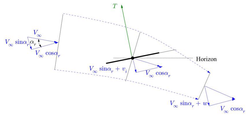
Figure 3 Stream-tube scheme for forward flight.

New terms appear in the equations from the balances: the rotor inclination angle ( α r ) MathType@MTEF@5@5@+= feaagKart1ev2aaatCvAUfeBSjuyZL2yd9gzLbvyNv2CaerbuLwBLn hiov2DGi1BTfMBaeXatLxBI9gBaerbd9wDYLwzYbItLDharqqtubsr 4rNCHbGeaGqk0dg9crFfpeea0xh9v8qiW7rqqrFfpeea0xe9Lq=Jc9 vqaqpepm0xbba9pwe9Q8fs0=yqaqpepae9pg0FirpepeKkFr0xfr=x fr=xb9adbaqaaeGaciGaaiaabeqaamaabaabaaGcbaaeaaaaaaaaa8 qadaqadaWdaeaapeGaeqySde2damaaBaaaleaapeGaamOCaaWdaeqa aaGcpeGaayjkaiaawMcaaaaa@3CE3@ and the advance speed of the vehicle ( V ) MathType@MTEF@5@5@+= feaagKart1ev2aaatCvAUfeBSjuyZL2yd9gzLbvyNv2CaerbuLwBLn hiov2DGi1BTfMBaeXatLxBI9gBaerbd9wDYLwzYbItLDharqqtubsr 4rNCHbGeaGqk0dg9crFfpeea0xh9v8qiW7rqqrFfpeea0xe9Lq=Jc9 vqaqpepm0xbba9pwe9Q8fs0=yqaqpepae9pg0FirpepeKkFr0xfr=x fr=xb9adbaqaaeGaciGaaiaabeqaamaabaabaaGcbaaeaaaaaaaaa8 qadaqadaWdaeaapeGaamOva8aadaWgaaWcbaWdbiabg6HiLcWdaeqa aaGcpeGaayjkaiaawMcaaaaa@3C99@ .

V= ( V sin α r + v i ) 2 + ( V cos α r ) 2  T=m( V sin α r  + w ˙ ) m ˙ V sin α r T( V sin α r + v i )= 1 2 m ˙ ( V 2 V 2 ) w=2 v i MathType@MTEF@5@5@+= feaagKart1ev2aaatCvAUfeBSjuyZL2yd9gzLbvyNv2CaerbuLwBLn hiov2DGi1BTfMBaeXatLxBI9gBaerbd9wDYLwzYbItLDharqqtubsr 4rNCHbGeaGqk0dg9crFfpeea0xh9v8qiW7rqqrFfpeea0xe9Lq=Jc9 vqaqpepm0xbba9pwe9Q8fs0=yqaqpepae9pg0FirpepeKkFr0xfr=x fr=xb9adbaqaaeGaciGaaiaabeqaamaabaabaaGceaqabeaaqaaaaa aaaaWdbiaadAfacqGH9aqpdaGcaaWdaeaapeWaaeWaa8aabaWdbiaa dAfapaWaaSbaaSqaa8qacqGHEisPa8aabeaak8qacaWGZbGaamyAai aad6gacqaHXoqypaWaaSbaaSqaa8qacaWGYbaapaqabaGcpeGaey4k aSIaamODa8aadaWgaaWcbaWdbiaadMgaa8aabeaaaOWdbiaawIcaca GLPaaapaWaaWbaaSqabeaapeGaaGOmaaaakiabgUcaRmaabmaapaqa a8qacaWGwbWdamaaBaaaleaapeGaeyOhIukapaqabaGcpeGaam4yai aad+gacaWGZbGaeqySde2damaaBaaaleaapeGaamOCaaWdaeqaaaGc peGaayjkaiaawMcaa8aadaahaaWcbeqaa8qacaaIYaaaaaqabaaake aacaGGGcGaamivaiabg2da9iaad2gadaqadaWdaeaapeGaamOva8aa daWgaaWcbaWdbiabg6HiLcWdaeqaaOWdbiaadohacaWGPbGaamOBai abeg7aH9aadaWgaaWcbaWdbiaadkhaa8aabeaak8qacaGGGcGaey4k aSIabm4DayaacaaacaGLOaGaayzkaaGaeyOeI0IabmyBa8aagaGaa8 qacaWGwbWdamaaBaaaleaapeGaeyOhIukapaqabaGcpeGaam4Caiaa dMgacaWGUbGaeqySde2damaaBaaaleaapeGaamOCaaWdaeqaaaGcba WdbiaadsfadaqadaWdaeaapeGaamOva8aadaWgaaWcbaWdbiabg6Hi LcWdaeqaaOWdbiaadohacaWGPbGaamOBaiabeg7aH9aadaWgaaWcba Wdbiaadkhaa8aabeaak8qacqGHRaWkcaWG2bWdamaaBaaaleaapeGa amyAaaWdaeqaaaGcpeGaayjkaiaawMcaaiabg2da9maalaaapaqaa8 qacaaIXaaapaqaa8qacaaIYaaaaiqad2gapaGbaiaapeWaaeWaa8aa baWdbiaadAfapaWaaWbaaSqabeaapeGaaGOmaaaakiabgkHiTiaadA fapaWaa0baaSqaa8qacqGHEisPa8aabaWdbiaaikdaaaaakiaawIca caGLPaaaaeaacaWG3bGaeyypa0JaaGOmaiaadAhapaWaaSbaaSqaa8 qacaWGPbaapaqabaaaaaa@905D@ (2)

Blade element theory (BET)

Momentum theory does not consider any aspect related with rotor geometry except for the radius. The estimations are based on conservation laws and not on aerodynamic principles neglecting viscosity, hence drag forces and parasite power cannot be computed. BET computes rotors forces, torque (Q) and power, induced and parasite ( P i ,   P 0 ) MathType@MTEF@5@5@+= feaagKart1ev2aaatCvAUfeBSjuyZL2yd9gzLbvyNv2CaerbuLwBLn hiov2DGi1BTfMBaeXatLxBI9gBaerbd9wDYLwzYbItLDharqqtubsr 4rNCHbGeaGqk0dg9crFfpeea0xh9v8qiW7rqqrFfpeea0xe9Lq=Jc9 vqaqpepm0xbba9pwe9Q8fs0=yqaqpepae9pg0FirpepeKkFr0xfr=x fr=xb9adbaqaaeGaciGaaiaabeqaamaabaabaaGcbaaeaaaaaaaaa8 qadaqadaWdaeaapeGaamiua8aadaWgaaWcbaWdbiaadMgaa8aabeaa k8qacaGGSaGaaiiOaiaacckacaWGqbWdamaaBaaaleaapeGaaGimaa WdaeqaaaGcpeGaayjkaiaawMcaaaaa@410B@ , based on 2-D theory using the aerodynamic forces at each blade section and integrating along the blade. Only some 3-D effects can be implemented by modifications of the theory.

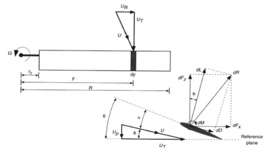
Figure 4, shows the velocities over the blade section, radial ( U R ) MathType@MTEF@5@5@+= feaagKart1ev2aaatCvAUfeBSjuyZL2yd9gzLbvyNv2CaerbuLwBLn hiov2DGi1BTfMBaeXatLxBI9gBaerbd9wDYLwzYbItLDharqqtubsr 4rNCHbGeaGqk0dg9crFfpeea0xh9v8qiW7rqqrFfpeea0xe9Lq=Jc9 vqaqpepm0xbba9pwe9Q8fs0=yqaqpepae9pg0FirpepeKkFr0xfr=x fr=xb9adbaqaaeGaciGaaiaabeqaamaabaabaaGcbaaeaaaaaaaaa8 qadaqadaWdaeaapeGaamyva8aadaWgaaWcbaWdbiaadkfaa8aabeaa aOWdbiaawIcacaGLPaaaaaa@3BFE@ , which is neglected, tangential ( U T ) MathType@MTEF@5@5@+= feaagKart1ev2aaatCvAUfeBSjuyZL2yd9gzLbvyNv2CaerbuLwBLn hiov2DGi1BTfMBaeXatLxBI9gBaerbd9wDYLwzYbItLDharqqtubsr 4rNCHbGeaGqk0dg9crFfpeea0xh9v8qiW7rqqrFfpeea0xe9Lq=Jc9 vqaqpepm0xbba9pwe9Q8fs0=yqaqpepae9pg0FirpepeKkFr0xfr=x fr=xb9adbaqaaeGaciGaaiaabeqaamaabaabaaGcbaaeaaaaaaaaa8 qadaqadaWdaeaapeGaamyva8aadaWgaaWcbaGaamivaaqabaaak8qa caGLOaGaayzkaaaaaa@3BE1@ and perpendicular ( U P ) MathType@MTEF@5@5@+= feaagKart1ev2aaatCvAUfeBSjuyZL2yd9gzLbvyNv2CaerbuLwBLn hiov2DGi1BTfMBaeXatLxBI9gBaerbd9wDYLwzYbItLDharqqtubsr 4rNCHbGeaGqk0dg9crFfpeea0xh9v8qiW7rqqrFfpeea0xe9Lq=Jc9 vqaqpepm0xbba9pwe9Q8fs0=yqaqpepae9pg0FirpepeKkFr0xfr=x fr=xb9adbaqaaeGaciGaaiaabeqaamaabaabaaGcbaaeaaaaaaaaa8 qadaqadaWdaeaapeGaamyva8aadaWgaaWcbaGaamiuaaqabaaak8qa caGLOaGaayzkaaaaaa@3BDD@ as well as the differential forces ( d F z ,d F x ) MathType@MTEF@5@5@+= feaagKart1ev2aaatCvAUfeBSjuyZL2yd9gzLbvyNv2CaerbuLwBLn hiov2DGi1BTfMBaeXatLxBI9gBaerbd9wDYLwzYbItLDharqqtubsr 4rNCHbGeaGqk0dg9crFfpeea0xh9v8qiW7rqqrFfpeea0xe9Lq=Jc9 vqaqpepm0xbba9pwe9Q8fs0=yqaqpepae9pg0FirpepeKkFr0xfr=x fr=xb9adbaqaaeGaciGaaiaabeqaamaabaabaaGcbaaeaaaaaaaaa8 qadaqadaWdaeaapeGaamizaiaadAeapaWaaSbaaSqaa8qacaWG6baa paqabaGcpeGaaiilaiaadsgacaWGgbWdamaaBaaaleaapeGaamiEaa WdaeqaaaGcpeGaayjkaiaawMcaaaaa@40D5@ and the aerodynamic terms lift, drag and moment (L,D,M). Additionally, it appears the geometrical pitch ( θ ) MathType@MTEF@5@5@+= feaagKart1ev2aaatCvAUfeBSjuyZL2yd9gzLbvyNv2CaerbuLwBLn hiov2DGi1BTfMBaeXatLxBI9gBaerbd9wDYLwzYbItLDharqqtubsr 4rNCHbGeaGqk0dg9crFfpeea0xh9v8qiW7rqqrFfpeea0xe9Lq=Jc9 vqaqpepm0xbba9pwe9Q8fs0=yqaqpepae9pg0FirpepeKkFr0xfr=x fr=xb9adbaqaaeGaciGaaiaabeqaamaabaabaaGcbaaeaaaaaaaaa8 qadaqadaWdaeaapeGaeqiUdehacaGLOaGaayzkaaaaaa@3B8F@ , the angle of attack ( α ) MathType@MTEF@5@5@+= feaagKart1ev2aaatCvAUfeBSjuyZL2yd9gzLbvyNv2CaerbuLwBLn hiov2DGi1BTfMBaeXatLxBI9gBaerbd9wDYLwzYbItLDharqqtubsr 4rNCHbGeaGqk0dg9crFfpeea0xh9v8qiW7rqqrFfpeea0xe9Lq=Jc9 vqaqpepm0xbba9pwe9Q8fs0=yqaqpepae9pg0FirpepeKkFr0xfr=x fr=xb9adbaqaaeGaciGaaiaabeqaamaabaabaaGcbaaeaaaaaaaaa8 qadaqadaWdaeaacqaHXoqya8qacaGLOaGaayzkaaaaaa@3B78@ and the inflow angle ( ϕ ) MathType@MTEF@5@5@+= feaagKart1ev2aaatCvAUfeBSjuyZL2yd9gzLbvyNv2CaerbuLwBLn hiov2DGi1BTfMBaeXatLxBI9gBaerbd9wDYLwzYbItLDharqqtubsr 4rNCHbGeaGqk0dg9crFfpeea0xh9v8qiW7rqqrFfpeea0xe9Lq=Jc9 vqaqpepm0xbba9pwe9Q8fs0=yqaqpepae9pg0FirpepeKkFr0xfr=x fr=xb9adbaqaaeGaciGaaiaabeqaamaabaabaaGcbaaeaaaaaaaaa8 qadaqadaWdaeaacqaHvpGza8qacaGLOaGaayzkaaaaaa@3BA1@ as well as the non-dimensional radius ( r=y/R ) MathType@MTEF@5@5@+= feaagKart1ev2aaatCvAUfeBSjuyZL2yd9gzLbvyNv2CaerbuLwBLn hiov2DGi1BTfMBaeXatLxBI9gBaerbd9wDYLwzYbItLDharqqtubsr 4rNCHbGeaGqk0dg9crFfpeea0xh9v8qiW7rqqrFfpeea0xe9Lq=Jc9 vqaqpepm0xbba9pwe9Q8fs0=yqaqpepae9pg0FirpepeKkFr0xfr=x fr=xb9adbaqaaeGaciGaaiaabeqaamaabaabaaGcbaaeaaaaaaaaa8 qadaqadaWdaeaapeGaamOCaiabg2da9iaadMhacaGGVaGaamOuaaGa ayjkaiaawMcaaaaa@3E5E@ . By composition of those forces, the expressions that integrated along the blade provide the final computation are reached.

U P = v i ,  U T =ΩrR, α=θϕϕ=atan( U P U T ) MathType@MTEF@5@5@+= feaagKart1ev2aaatCvAUfeBSjuyZL2yd9gzLbvyNv2CaerbuLwBLn hiov2DGi1BTfMBaeXatLxBI9gBaerbd9wDYLwzYbItLDharqqtubsr 4rNCHbGeaGqk0dg9crFfpeea0xh9v8qiW7rqqrFfpeea0xe9Lq=Jc9 vqaqpepm0xbba9pwe9Q8fs0=yqaqpepae9pg0FirpepeKkFr0xfr=x fr=xb9adbaqaaeGaciGaaiaabeqaamaabaabaaGcbaqcLbsaqaaaaa aaaaWdbiaadwfak8aadaWgaaWcbaqcLbmapeGaamiuaaWcpaqabaqc LbsapeGaeyypa0JaamODaSWdamaaBaaabaqcLbmapeGaamyAaaWcpa qabaqcLbsapeGaaiilaiaacckacaWGvbWcpaWaaSbaaeaajugWa8qa caWGubaal8aabeaajugib8qacqGH9aqpcaqGPoGaaeOCaiaadkfaca GGSaGaaiiOaiabeg7aHjabg2da9iabeI7aXjabgkHiTiabew9aMjab gkziUkabew9aMjabg2da9iaabggacaqG0bGaaeyyaiaab6gakmaabm aapaqaa8qadaWcaaWdaeaajugib8qacaWGvbWcpaWaaSbaaeaajugW a8qacaWGqbaal8aabeaaaOqaaKqzGeWdbiaadwfal8aadaWgaaqaaK qzadWdbiaadsfaaSWdaeqaaaaaaOWdbiaawIcacaGLPaaaaaa@6690@ (3)

Lift and drag are computed using the dynamic pressure ( 1/2ρ U 2 ) MathType@MTEF@5@5@+= feaagKart1ev2aqatCvAUfeBSjuyZL2yd9gzLbvyNv2CaerbuLwBLn hiov2DGi1BTfMBaeXatLxBI9gBaerbd9wDYLwzYbItLDharqqtubsr 4rNCHbGeaGqk0dg9crFfpeea0xh9v8qiW7rqqrFfpeea0xe9Lq=Jc9 vqaqpepm0xbba9pwe9Q8fs0=yqaqpepae9pg0FirpepeKkFr0xfr=x fr=xb9adbaqaaeGaciGaaiaabeqaamaabaabaaGcbaaeaaaaaaaaa8 qadaqadaqaaiaaigdacaGGVaGaaGOmaiabeg8aYjaadwfapaWaaWba aSqabeaapeGaaGOmaaaaaOGaayjkaiaawMcaaaaa@3F91@ , the chord distribution (c) and the airfoil properties: lift and drag coefficient (Cl,Cd).

dL= 1 2 ρ U 2 Clcdy,dD= 1 2 ρ U 2 Ccdy d F z =dLcosϕdDsinϕ,   d F x =dLsinϕ+dDcosϕ MathType@MTEF@5@5@+= feaagKart1ev2aqatCvAUfeBSjuyZL2yd9gzLbvyNv2CaerbuLwBLn hiov2DGi1BTfMBaeXatLxBI9gBaerbd9wDYLwzYbItLDharqqtubsr 4rNCHbGeaGqk0dg9crFfpeea0xh9v8qiW7rqqrFfpeea0xe9Lq=Jc9 vqaqpepm0xbba9pwe9Q8fs0=yqaqpepae9pg0FirpepeKkFr0xfr=x fr=xb9adbaqaaeGaciGaaiaabeqaamaabaabaaGceaqabeaaqaaaaa aaaaWdbiaadsgacaWGmbGaeyypa0ZaaSaaaeaacaaIXaaabaGaaGOm aaaacqaHbpGCcaWGvbWdamaaCaaaleqabaWdbiaaikdaaaGccaWGdb GaamiBaiaadogacaWGKbGaamyEaiaacYcacaWGKbGaamiraiabg2da 9maalaaabaGaaGymaaqaaiaaikdaaaGaeqyWdiNaamyva8aadaahaa Wcbeqaa8qacaaIYaaaaOGaam4qaiaadogacaWGKbGaamyEaaqaaiaa dsgacaWGgbWdamaaBaaaleaapeGaamOEaaWdaeqaaOWdbiabg2da9i aadsgacaWGmbGaam4yaiaad+gacaWGZbGaeqy1dyMaeyOeI0Iaamiz aiaadseacaWGZbGaamyAaiaad6gacqaHvpGzcaGGSaGaaiiOaiaacc kacaGGGcGaamizaiaadAeapaWaaSbaaSqaa8qacaWG4baapaqabaGc peGaeyypa0JaamizaiaadYeacaWGZbGaamyAaiaad6gacqaHvpGzcq GHRaWkcaWGKbGaamiraiaadogacaWGVbGaam4Caiabew9aMbaaaa@787B@ (4)

Finally, differential expressions of thrust, torque and power are obtained using the number of blades (b) and the rotational speed (Ω).

dT=bd F z , dQ=bd F x rR, dP=bd F x ΩrR MathType@MTEF@5@5@+= feaagKart1ev2aaatCvAUfeBSjuyZL2yd9gzLbvyNv2CaerbuLwBLn hiov2DGi1BTfMBaeXatLxBI9gBaerbd9wDYLwzYbItLDharqqtubsr 4rNCHbGeaGqk0dg9crFfpeea0xh9v8qiW7rqqrFfpeea0xe9Lq=Jc9 vqaqpepm0xbba9pwe9Q8fs0=yqaqpepae9pg0FirpepeKkFr0xfr=x fr=xb9adbaqaaeGaciGaaiaabeqaamaabaabaaGcbaqcLbsaqaaaaa aaaaWdbiaadsgacaWGubGaeyypa0JaamOyaiaadsgacaWGgbGcpaWa aSbaaSqaaKqzGeWdbiaadQhaaSWdaeqaaKqzGeWdbiaacYcacaGGGc GaamizaiaadgfacqGH9aqpcaWGIbGaamizaiaadAeak8aadaWgaaWc baqcLbsapeGaamiEaaWcpaqabaqcLbsapeGaamOCaiaadkfacaGGSa GaaiiOaiaadsgacaWGqbGaeyypa0JaamOyaiaadsgacaWGgbGcpaWa aSbaaSqaaKqzGeWdbiaadIhaaSWdaeqaaKqzGeWdbiaabM6acaWGYb GaamOuaaaa@5925@ (5)

Frequently, these final expressions are non-diomensionalized using the rotor area ( A r ) MathType@MTEF@5@5@+= feaagKart1ev2aqatCvAUfeBSjuyZL2yd9gzLbvyNv2CaerbuLwBLn hiov2DGi1BTfMBaeXatLxBI9gBaerbd9wDYLwzYbItLDharqqtubsr 4rNCHbGeaGqk0dg9crFfpeea0xh9v8qiW7rqqrFfpeea0xe9Lq=Jc9 vqaqpepm0xbba9pwe9Q8fs0=yqaqpepae9pg0FirpepeKkFr0xfr=x fr=xb9adbaqaaeGaciGaaiaabeqaamaabaabaaGcbaWaaeWaaeaaqa aaaaaaaaWdbiaadgeapaWaaSbaaSqaa8qacaWGYbaapaqabaaakiaa wIcacaGLPaaaaaa@3BDC@ , the tip speed ( ΩR ) MathType@MTEF@5@5@+= feaagKart1ev2aqatCvAUfeBSjuyZL2yd9gzLbvyNv2CaerbuLwBLn hiov2DGi1BTfMBaeXatLxBI9gBaerbd9wDYLwzYbItLDharqqtubsr 4rNCHbGeaGqk0dg9crFfpeea0xh9v8qiW7rqqrFfpeea0xe9Lq=Jc9 vqaqpepm0xbba9pwe9Q8fs0=yqaqpepae9pg0FirpepeKkFr0xfr=x fr=xb9adbaqaaeGaciGaaiaabeqaamaabaabaaGcbaWaaeWaaeaaju gibabaaaaaaaaapeGaaeyQdiaabkfaaOWdaiaawIcacaGLPaaaaaa@3C67@ and new parameters, the solidity ( σ=( bc )/( πR ) ) MathType@MTEF@5@5@+= feaagKart1ev2aaatCvAUfeBSjuyZL2yd9gzLbvyNv2CaerbuLwBLn hiov2DGi1BTfMBaeXatLxBI9gBaerbd9wDYLwzYbItLDharqqtubsr 4rNCHbGeaGqk0dg9crFfpeea0xh9v8qiW7rqqrFfpeea0xe9Lq=Jc9 vqaqpepm0xbba9pwe9Q8fs0=yqaqpepae9pg0FirpepeKkFr0xfr=x fr=xb9adbaqaaeGaciGaaiaabeqaamaabaabaaGcbaaeaaaaaaaaa8 qadaqadaWdaeaapeGaeq4WdmNaeyypa0ZaaeWaa8aabaWdbiaadkga caWGJbaacaGLOaGaayzkaaGaai4lamaabmaapaqaa8qacqaHapaCca WGsbaacaGLOaGaayzkaaaacaGLOaGaayzkaaaaaa@4508@ and the inflow parameter ( λ=U P /( ΩR ) ) MathType@MTEF@5@5@+= feaagKart1ev2aqatCvAUfeBSjuyZL2yd9gzLbvyNv2CaerbuLwBLn hiov2DGi1BTfMBaeXatLxBI9gBaerbd9wDYLwzYbItLDharqqtubsr 4rNCHbGeaGqk0dg9crFfpeea0xh9v8qiW7rqqrFfpeea0xe9Lq=Jc9 vqaqpepm0xbba9pwe9Q8fs0=yqaqpepae9pg0FirpepeKkFr0xfr=x fr=xb9adbaqaaeGaciGaaiaabeqaamaabaabaaGcbaaeaaaaaaaaa8 qadaqadaWdaeaajugib8qacaqG7oGaaeypaiaabwfak8aadaWgaaWc baqcLbmapeGaaeiuaaWcpaqabaqcLbsapeGaae4laOWaaeWaa8aaba qcLbsapeGaaeyQdiaabkfaaOGaayjkaiaawMcaaaGaayjkaiaawMca aaaa@4552@ .

d C T = dT 2ρ A r ( ΩR ) 2   = 1 2 σ( Clcosf-Cdsinf )( r 2 + λ 2 )dr d C P = dP 2ρ A r ( ΩR ) 3   = 1 2 σ( Clsinf+Cdcosf )( r 2 + λ 2 )rdrΑ MathType@MTEF@5@5@+= feaagKart1ev2aqatCvAUfeBSjuyZL2yd9gzLbvyNv2CaerbuLwBLn hiov2DGi1BTfMBaeXatLxBI9gBaerbd9wDYLwzYbItLDharqqtubsr 4rNCHbGeaGqk0dg9crFfpeea0xh9v8qiW7rqqrFfpeea0xe9Lq=Jc9 vqaqpepm0xbba9pwe9Q8fs0=yqaqpepae9pg0FirpepeKkFr0xfr=x fr=xb9adbaqaaeGaciGaaiaabeqaamaabaabaaGceaqabeaajugiba baaaaaaaaapeGaamizaiaadoeak8aadaWgaaWcbaqcLbmapeGaamiv aaWcpaqabaqcLbsapeGaeyypa0JcdaWcaaWdaeaajugib8qacaWGKb GaamivaaGcpaqaaKqzGeWdbiaaikdacqaHbpGCcaWGbbWcpaWaaSba aeaajugWa8qacaWGYbaal8aabeaak8qadaqadaWdaeaajugib8qaca qGPoGaamOuaaGccaGLOaGaayzkaaWdamaaCaaaleqabaqcLbmapeGa aGOmaaaajugibiaacckaaaGaeyypa0JcdaWcaaWdaeaajugib8qaca aIXaaak8aabaqcLbsapeGaaGOmaaaacqaHdpWCkmaabmaapaqaaKqz GeWdbiaadoeacaWGSbGaci4yaiaac+gacaGGZbGaamOzaiaac2caca WGdbGaamizaiGacohacaGGPbGaaiOBaiaadAgaaOGaayjkaiaawMca amaabmaapaqaaKqzGeWdbiaadkhak8aadaahaaWcbeqaaKqzadWdbi aaikdaaaqcLbsacqGHRaWkcqaH7oaBl8aadaahaaqabeaajugWa8qa caaIYaaaaaGccaGLOaGaayzkaaqcLbsacaWGKbGaamOCaaGcbaqcLb sacaWGKbGaam4qaSWdamaaBaaabaqcLbmapeGaamiuaaWcpaqabaqc LbsapeGaeyypa0JcdaWcaaWdaeaajugib8qacaWGKbGaamiuaaGcpa qaaKqzGeWdbiaaikdacqaHbpGCcaWGbbGcpaWaaSbaaSqaaKqzGeWd biaadkhaaSWdaeqaaOWdbmaabmaapaqaaKqzGeWdbiaabM6acaWGsb aakiaawIcacaGLPaaapaWaaWbaaSqabeaajugWa8qacaaIZaaaaKqz GeGaaiiOaaaacqGH9aqpkmaalaaapaqaaKqzGeWdbiaaigdaaOWdae aajugib8qacaaIYaaaaiabeo8aZPWaaeWaa8aabaqcLbsapeGaam4q aiaadYgaciGGZbGaaiyAaiaac6gacaWGMbGaey4kaSIaam4qaiaads gaciGGJbGaai4BaiaacohacaWGMbaakiaawIcacaGLPaaadaqadaWd aeaajugib8qacaWGYbWcpaWaaWbaaeqabaqcLbmapeGaaGOmaaaaju gibiabgUcaRiabeU7aSTWdamaaCaaabeqaaKqzadWdbiaaikdaaaaa kiaawIcacaGLPaaajugibiaadkhacaWGKbGaamOCaiabfg5abbaaaa@AB53@ (6)

Figure 4 Blade Element theory model, forces, and velocities at the blade section.16

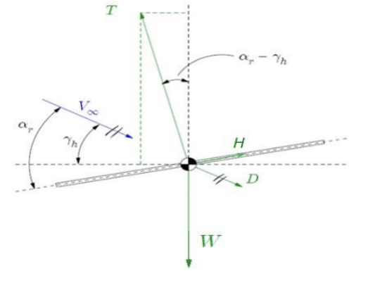
Similarly to momentum theory, BET can be applied in forward flight. The main difference is the velocity field and the forces, Figure 5. At forward flight, velocity field is not axisymmetric, the magnitudes must be averaged in a revolution because they depend on the azimuth position (ψ).

Whereas the expressions of lift and drag forces do not change from equation 4, tangential and perpendicular speeds do, as well as the final forces. Moreover, the axial force ( F x ) MathType@MTEF@5@5@+= feaagKart1ev2aqatCvAUfeBSjuyZL2yd9gzLbvyNv2CaerbuLwBLn hiov2DGi1BTfMBaeXatLxBI9gBaerbd9wDYLwzYbItLDharqqtubsr 4rNCHbGeaGqk0dg9crFfpeea0xh9v8qiW7rqqrFfpeea0xe9Lq=Jc9 vqaqpepm0xbba9pwe9Q8fs0=yqaqpepae9pg0FirpepeKkFr0xfr=x fr=xb9adbaqaaeGaciGaaiaabeqaamaabaabaaGcbaWaaeWaaeaaqa aaaaaaaaWdbiaadAeapaWaaSbaaSqaa8qacaWG4baapaqabaaakiaa wIcacaGLPaaaaaa@3BE7@ of the previous scheme, which is denominated as dragging force, is split in two (Y,H). Apart from that, functions ( F t ,  F h ) MathType@MTEF@5@5@+= feaagKart1ev2aaatCvAUfeBSjuyZL2yd9gzLbvyNv2CaerbuLwBLn hiov2DGi1BTfMBaeXatLxBI9gBaerbd9wDYLwzYbItLDharqqtubsr 4rNCHbGeaGqk0dg9crFfpeea0xh9v8qiW7rqqrFfpeea0xe9Lq=Jc9 vqaqpepm0xbba9pwe9Q8fs0=yqaqpepae9pg0FirpepeKkFr0xfr=x fr=xb9adbaqaaeGaciGaaiaabeqaamaabaabaaGcbaWaaeWaaeaaqa aaaaaaaaWdbiaadAeapaWaaSbaaSqaa8qacaWG0baapaqabaGcpeGa aiilaiaacckacaWGgbWdamaaBaaaleaapeGaamiAaaWdaeqaaaGcca GLOaGaayzkaaaaaa@3FE2@ are implemented for quantifying losses at the tip and hub, more information about them is available in.16

U P = V sin α r + v i ,      U T =Ωr+ V cos α r sinψ dCT= 1 2 σ( ClcosϕCdsinϕ ) U 2 F t F h dr dCQ=dCP= 1 2 σ( Clsinϕ+Cdcosϕ ) U 2 rdr dCY= 1 2 σ( Clsinϕ+Cdcosϕ ) U 2 cosψdr dCH= 1 2 σ( Clsinϕ+Cdcosϕ ) U 2 sinψdr MathType@MTEF@5@5@+= feaagKart1ev2aaatCvAUfeBSjuyZL2yd9gzLbvyNv2CaerbuLwBLn hiov2DGi1BTfMBaeXatLxBI9gBaerbd9wDYLwzYbItLDharqqtubsr 4rNCHbGeaGqk0dg9crFfpeea0xh9v8qiW7rqqrFfpeea0xe9Lq=Jc9 vqaqpepm0xbba9pwe9Q8fs0=yqaqpepae9pg0FirpepeKkFr0xfr=x fr=xb9adbaqaaeGaciGaaiaabeqaamaabaabaaGceaqabeaaqaaaaa aaaaWdbiaadwfapaWaaSbaaSqaa8qacaWGqbaapaqabaGcpeGaeyyp a0JaamOva8aadaWgaaWcbaWdbiabg6HiLcWdaeqaaOWdbiaadohaca WGPbGaamOBaiabeg7aH9aadaWgaaWcbaWdbiaadkhaa8aabeaak8qa cqGHRaWkcaWG2bWdamaaBaaaleaapeGaamyAaaWdaeqaaOWdbiaacY cacaGGGcGaaiiOaiaacckacaGGGcGaaiiOaiaadwfapaWaaSbaaSqa a8qacaWGubaapaqabaGcpeGaeyypa0JaeuyQdCLaamOCaiabgUcaRi aadAfapaWaaSbaaSqaa8qacqGHEisPa8aabeaak8qacaWGJbGaam4B aiaadohacqaHXoqypaWaaSbaaSqaa8qacaWGYbaapaqabaGcpeGaam 4CaiaadMgacaWGUbGaeqiYdKhabaGaamizaiaadoeacaWGubGaeyyp a0ZaaSaaa8aabaWdbiaaigdaa8aabaWdbiaaikdaaaGaeq4Wdm3aae Waa8aabaWdbiaadoeacaWGSbGaam4yaiaad+gacaWGZbGaeqy1dyMa eyOeI0Iaam4qaiaadsgacaWGZbGaamyAaiaad6gacqaHvpGzaiaawI cacaGLPaaacaWGvbWdamaaCaaaleqabaWdbiaaikdaaaGccaWGgbWd amaaBaaaleaapeGaamiDaaWdaeqaaOWdbiaadAeapaWaaSbaaSqaa8 qacaWGObaapaqabaGcpeGaamizaiaadkhaaeaacaWGKbGaam4qaiaa dgfacqGH9aqpcaWGKbGaam4qaiaadcfacqGH9aqpdaWcaaWdaeaape GaaGymaaWdaeaapeGaaGOmaaaacqaHdpWCdaqadaWdaeaapeGaam4q aiaadYgacaWGZbGaamyAaiaad6gacqaHvpGzcqGHRaWkcaWGdbGaam izaiaadogacaWGVbGaam4Caiabew9aMbGaayjkaiaawMcaaiaadwfa paWaaWbaaSqabeaapeGaaGOmaaaakiaadkhacaWGKbGaamOCaaqaai aadsgacaWGdbGaamywaiabg2da9maalaaapaqaa8qacaaIXaaapaqa a8qacaaIYaaaaiabeo8aZnaabmaapaqaa8qacaWGdbGaamiBaiaado hacaWGPbGaamOBaiabew9aMjabgUcaRiaadoeacaWGKbGaam4yaiaa d+gacaWGZbGaeqy1dygacaGLOaGaayzkaaGaamyva8aadaahaaWcbe qaa8qacaaIYaaaaOGaci4yaiaac+gacaGGZbGaeqiYdKNaamizaiaa dkhaaeaacaWGKbGaam4qaiaadIeacqGH9aqpdaWcaaWdaeaapeGaaG ymaaWdaeaapeGaaGOmaaaacqaHdpWCdaqadaWdaeaapeGaam4qaiaa dYgacaWGZbGaamyAaiaad6gacqaHvpGzcqGHRaWkcaWGdbGaamizai aadogacaWGVbGaam4Caiabew9aMbGaayjkaiaawMcaaiaadwfapaWa aWbaaSqabeaapeGaaGOmaaaakiaadohacaWGPbGaamOBaiabeI8a5j aadsgacaWGYbaaaaa@DC07@ (7)

Frequently, the theory is simplified assuming small angles, tangential speed much bigger than perpendicular speed and high Reynolds simplifications ( ClC L α α,  ClCd ) MathType@MTEF@5@5@+= feaagKart1ev2aqatCvAUfeBSjuyZL2yd9gzLbvyNv2CaerbuLwBLn hiov2DGi1BTfMBaeXatLxBI9gBaerbd9wDYLwzYbItLDharqqtubsr 4rNCHbGeaGqk0dg9crFfpeea0xh9v8qiW7rqqrFfpeea0xe9Lq=Jc9 vqaqpepm0xbba9pwe9Q8fs0=yqaqpepae9pg0FirpepeKkFr0xfr=x fr=xb9adbaqaaeGaciGaaiaabeqaamaabaabaaGcbaaeaaaaaaaaa8 qadaqadaWdaeaapeGaam4qaiaadYgacqGHijYUcaWGdbGaamita8aa daWgaaWcbaWdbiabeg7aHbWdaeqaaOWdbiabeg7aHjaacYcacaGGGc GaaiiOaiaadoeacaWGSbGaeSOAI0Jaam4qaiaadsgaaiaawIcacaGL Paaaaaa@4A4B@ , which should not be applied for small scale rotors.

Figure 5 Blade Element theory scheme for forward flight, forces, and velocities at the blade section.

Blade element and momentum theory 

As subjected, BET considers geometrical blade parameters for computing the total power of the rotor. However, the induced speed or the inflow (λ) required for the computation must be provided whereas the momentum theory estimates it using the thrust. The momentum theory applied in differential form,16 (annular sections), combined with BET creates the final approach used for the computations, the blade element and momentum theory (BEMT), using the equality of the expressions of thrust coefficient (CT) provided by BET and differential momentum theory.

dCT= σ 2 C l α ( θ λ r ) r 2 dr=4 λ 2 F t F h rdr λ= σC l α 16 + σC l α 16 + σC l α θr 8 F t F h MathType@MTEF@5@5@+= feaagKart1ev2aqatCvAUfeBSjuyZL2yd9gzLbvyNv2CaerbuLwBLn hiov2DGi1BTfMBaeXatLxBI9gBaerbd9wDYLwzYbItLDharqqtubsr 4rNCHbGeaGqk0dg9crFfpeea0xh9v8qiW7rqqrFfpeea0xe9Lq=Jc9 vqaqpepm0xbba9pwe9Q8fs0=yqaqpepae9pg0FirpepeKkFr0xfr=x fr=xb9adbaqaaeGaciGaaiaabeqaamaabaabaaGceaqabeaaqaaaaa aaaaWdbiaadsgacaWGdbGaamivaiabg2da9maalaaapaqaa8qacqaH dpWCa8aabaWdbiaaikdaaaGaam4qaiaadYgapaWaaSbaaSqaa8qacq aHXoqya8aabeaak8qadaqadaWdaeaapeGaeqiUdeNaeyOeI0YaaSaa a8aabaWdbiabeU7aSbWdaeaapeGaamOCaaaaaiaawIcacaGLPaaaca WGYbWdamaaCaaaleqabaWdbiaaikdaaaGccaWGKbGaamOCaiabg2da 9iaaisdacqaH7oaBpaWaaWbaaSqabeaapeGaaGOmaaaakiaadAeapa WaaSbaaSqaa8qacaWG0baapaqabaGcpeGaamOra8aadaWgaaWcbaWd biaadIgaa8aabeaak8qacaWGYbGaamizaiaadkhaaeaacqaH7oaBcq GH9aqpcqGHsisldaWcaaWdaeaapeGaeq4WdmNaam4qaiaadYgapaWa aSbaaSqaa8qacqaHXoqya8aabeaaaOqaa8qacaaIXaGaaGOnaaaacq GHRaWkdaGcaaWdaeaapeWaaSaaa8aabaWdbiabeo8aZjaadoeacaWG SbWdamaaBaaaleaapeGaeqySdegapaqabaaakeaapeGaaGymaiaaiA daaaGaey4kaSYaaSaaa8aabaWdbiabeo8aZjaadoeacaWGSbWdamaa BaaaleaapeGaeqySdegapaqabaGcpeGaeqiUdeNaamOCaaWdaeaape GaaGioaiaadAeapaWaaSbaaSqaa8qacaWG0baapaqabaGcpeGaamOr a8aadaWgaaWcbaWdbiaadIgaa8aabeaaaaaapeqabaaaaaa@7B06@ (8)

Previous expression is obtained assuming the simplified form of BET and the differential momentum theory. Moreover, it takes into the account tip and hub 3-D losses with the functions ( F t ,  F h ) MathType@MTEF@5@5@+= feaagKart1ev2aaatCvAUfeBSjuyZL2yd9gzLbvyNv2CaerbuLwBLn hiov2DGi1BTfMBaeXatLxBI9gBaerbd9wDYLwzYbItLDharqqtubsr 4rNCHbGeaGqk0dg9crFfpeea0xh9v8qiW7rqqrFfpeea0xe9Lq=Jc9 vqaqpepm0xbba9pwe9Q8fs0=yqaqpepae9pg0FirpepeKkFr0xfr=x fr=xb9adbaqaaeGaciGaaiaabeqaamaabaabaaGcbaWaaeWaaeaaqa aaaaaaaaWdbiaadAeapaWaaSbaaSqaa8qacaWG0baapaqabaGcpeGa aiilaiaacckacaWGgbWdamaaBaaaleaapeGaamiAaaWdaeqaaaGcca GLOaGaayzkaaaaaa@3FE2@ , proposed by Prandtl and Lieshmann. More details about the functions can be found in.16 Besides that, the inflow can be expressed with the full BET, without linearization, as it is done in.6 However, during the validation, it was observed that for low Reynolds were drag can be high and NACA 0012 can generate even negative lift with positive angles, Figure 1, imaginary terms would appear making impossible to converge the solutions. To solvent that issue and still consider the non-linearity and the dependence with the Reynolds number, lift curves were approached with linear segments, Figure 6.

Equation 5 is applied modifying the pitch angle using the database with the slopes and the initial angles of each segment ( C l α , C l 0 ) MathType@MTEF@5@5@+= feaagKart1ev2aqatCvAUfeBSjuyZL2yd9gzLbvyNv2CaerbuLwBLn hiov2DGi1BTfMBaeXatLxBI9gBaerbd9wDYLwzYbItLDharqqtubsr 4rNCHbGeaGqk0dg9crFfpeea0xh9v8qiW7rqqrFfpeea0xe9Lq=Jc9 vqaqpepm0xbba9pwe9Q8fs0=yqaqpepae9pg0FirpepeKkFr0xfr=x fr=xb9adbaqaaeGaciGaaiaabeqaamaabaabaaGcbaaeaaaaaaaaa8 qadaqadaWdaeaapeGaam4qaiaadYgapaWaaSbaaSqaa8qacqaHXoqy a8aabeaak8qacaGGSaGaaiiOaiaadoeacaWGSbWdamaaBaaaleaape GaaGimaaWdaeqaaaGcpeGaayjkaiaawMcaaaaa@4261@ depending on the Reynolds at each section.

dCT= σ 2 C l α ( α+ C l o C l α )dr= σ 2 C l α ( θ λ r + C l 0 C l α ) r 2 dr θ =θ+C l 0 /C l α MathType@MTEF@5@5@+= feaagKart1ev2aqatCvAUfeBSjuyZL2yd9gzLbvyNv2CaerbuLwBLn hiov2DGi1BTfMBaeXatLxBI9gBaerbd9wDYLwzYbItLDharqqtubsr 4rNCHbGeaGqk0dg9crFfpeea0xh9v8qiW7rqqrFfpeea0xe9Lq=Jc9 vqaqpepm0xbba9pwe9Q8fs0=yqaqpepae9pg0FirpepeKkFr0xfr=x fr=xb9adbaqaaeGaciGaaiaabeqaamaabaabaaGcbaaeaaaaaaaaa8 qacaWGKbGaam4qaiaadsfacqGH9aqpdaWcaaWdaeaapeGaeq4Wdmha paqaa8qacaaIYaaaaiaadoeacaWGSbWdamaaBaaaleaapeGaeqySde gapaqabaGcpeWaaeWaa8aabaWdbiabeg7aHjabgUcaRmaalaaapaqa a8qacaWGdbGaamiBa8aadaWgaaWcbaWdbiaad+gaa8aabeaaaOqaa8 qacaWGdbGaamiBa8aadaWgaaWcbaWdbiabeg7aHbWdaeqaaaaaaOWd biaawIcacaGLPaaacaWGKbGaamOCaiabg2da9maalaaapaqaa8qacq aHdpWCa8aabaWdbiaaikdaaaGaam4qaiaadYgapaWaaSbaaSqaa8qa cqaHXoqya8aabeaak8qadaqadaWdaeaapeGaeqiUdeNaeyOeI0YaaS aaa8aabaWdbiabeU7aSbWdaeaapeGaamOCaaaacqGHRaWkdaWcaaWd aeaapeGaam4qaiaadYgapaWaaSbaaSqaa8qacaaIWaaapaqabaaake aapeGaam4qaiaadYgapaWaaSbaaSqaa8qacqaHXoqya8aabeaaaaaa k8qacaGLOaGaayzkaaGaamOCa8aadaahaaWcbeqaa8qacaaIYaaaaO GaamizaiaadkhacqGHsgIRcuaH4oqCpaGbauaapeGaeyypa0JaeqiU deNaey4kaSIaam4qaiaadYgapaWaaSbaaSqaa8qacaaIWaaapaqaba GcpeGaai4laiaadoeacaWGSbWdamaaBaaaleaapeGaeqySdegapaqa baaaaa@78C8@ (9)

Additionally, because of the tip and hub losses, the equation 5 is coupled. Hence, the problem must be solved using an iterative procedure as it is described in.1 Apart from that, the model can compute the required pilot input to provide a specific thrust or just to compute the thrust generated for a fixed configuration. The pilot input is typically the collective pitch but it was also considered the rotational speed (Ω), which is used for drones. The computation is performed using a numerical solution by Newton-Raphson with MATLAB fsolve function.

Glauert related the inflow at forward flight and hover16 so it was obtained an average inflow ( λ 0 ) MathType@MTEF@5@5@+= feaagKart1ev2aqatCvAUfeBSjuyZL2yd9gzLbvyNv2CaerbuLwBLn hiov2DGi1BTfMBaeXatLxBI9gBaerbd9wDYLwzYbItLDharqqtubsr 4rNCHbGeaGqk0dg9crFfpeea0xh9v8qiW7rqqrFfpeea0xe9Lq=Jc9 vqaqpepm0xbba9pwe9Q8fs0=yqaqpepae9pg0FirpepeKkFr0xfr=x fr=xb9adbaqaaeGaciGaaiaabeqaamaabaabaaGcbaaeaaaaaaaaa8 qadaqadaWdaeaapeGaeq4UdW2damaaBaaaleaapeGaaGimaaWdaeqa aaGcpeGaayjkaiaawMcaaaaa@3CBC@ from a biquadratic equation. Using the advance parameters ( μ x , μ y ) MathType@MTEF@5@5@+= feaagKart1ev2aqatCvAUfeBSjuyZL2yd9gzLbvyNv2CaerbuLwBLn hiov2DGi1BTfMBaeXatLxBI9gBaerbd9wDYLwzYbItLDharqqtubsr 4rNCHbGeaGqk0dg9crFfpeea0xh9v8qiW7rqqrFfpeea0xe9Lq=Jc9 vqaqpepm0xbba9pwe9Q8fs0=yqaqpepae9pg0FirpepeKkFr0xfr=x fr=xb9adbaqaaeGaciGaaiaabeqaamaabaabaaGcbaaeaaaaaaaaa8 qadaqadaWdaeaapeGaeqiVd02damaaBaaaleaapeGaamiEaaWdaeqa aOWdbiaacYcacqaH8oqBpaWaaSbaaSqaa8qacaWG5baapaqabaaak8 qacaGLOaGaayzkaaaaaa@40D9@ and the thrust coefficient (CT) and the induces inflow

( λ i = v i /( ΩR ) ) MathType@MTEF@5@5@+= feaagKart1ev2aaatCvAUfeBSjuyZL2yd9gzLbvyNv2CaerbuLwBLn hiov2DGi1BTfMBaeXatLxBI9gBaerbd9wDYLwzYbItLDharqqtubsr 4rNCHbGeaGqk0dg9crFfpeea0xh9v8qiW7rqqrFfpeea0xe9Lq=Jc9 vqaqpepm0xbba9pwe9Q8fs0=yqaqpepae9pg0FirpepeKkFr0xfr=x fr=xb9adbaqaaeGaciGaaiaabeqaamaabaabaaGcbaaeaaaaaaaaa8 qadaqadaWdaeaapeGaeq4UdW2damaaBaaaleaapeGaamyAaaWdaeqa aOWdbiabg2da9iaadAhapaWaaSbaaSqaa8qacaWGPbaapaqabaGcpe Gaai4lamaabmaapaqaa8qacaqGPoGaamOuaaGaayjkaiaawMcaaaGa ayjkaiaawMcaaaaa@44B3@ .

μ x = V cos α r ΩR ,    μ z = V sin α r ΩR ,    λ 0 = μ z + λ i λ i = CT 2 μ x 2 + λ 0 2 MathType@MTEF@5@5@+= feaagKart1ev2aaatCvAUfeBSjuyZL2yd9gzLbvyNv2CaerbuLwBLn hiov2DGi1BTfMBaeXatLxBI9gBaerbd9wDYLwzYbItLDharqqtubsr 4rNCHbGeaGqk0dg9crFfpeea0xh9v8qiW7rqqrFfpeea0xe9Lq=Jc9 vqaqpepm0xbba9pwe9Q8fs0=yqaqpepae9pg0FirpepeKkFr0xfr=x fr=xb9adbaqaaeGaciGaaiaabeqaamaabaabaaGceaqabeaaqaaaaa aaaaWdbiabeY7aT9aadaWgaaWcbaWdbiaadIhaa8aabeaak8qacqGH 9aqpdaWcaaWdaeaapeGaamOva8aadaWgaaWcbaWdbiabg6HiLcWdae qaaOWdbiaadogacaWGVbGaam4Caiabeg7aH9aadaWgaaWcbaWdbiaa dkhaa8aabeaaaOqaa8qacaqGPoGaaeOuaaaacaGGSaGaaiiOaiaacc kacaGGGcGaeqiVd02damaaBaaaleaapeGaamOEaaWdaeqaaOWdbiab g2da9maalaaapaqaa8qacaWGwbWdamaaBaaaleaapeGaeyOhIukapa qabaGcpeGaam4CaiaadMgacaWGUbGaeqySde2damaaBaaaleaapeGa amOCaaWdaeqaaaGcbaWdbiaabM6acaWGsbaaaiaacYcacaGGGcGaai iOaiaacckacqaH7oaBpaWaaSbaaSqaa8qacaaIWaaapaqabaGcpeGa eyypa0JaeqiVd02damaaBaaaleaapeGaamOEaaWdaeqaaOWdbiabgU caRiabeU7aS9aadaWgaaWcbaWdbiaadMgaa8aabeaaaOqaa8qacqaH 7oaBpaWaaSbaaSqaa8qacaWGPbaapaqabaGcpeGaeyypa0ZaaSaaa8 aabaWdbiaadoeacaWGubaapaqaa8qacaaIYaWaaOaaa8aabaWdbiab eY7aT9aadaqhaaWcbaWdbiaadIhaa8aabaWdbiaaikdaaaGccqGHRa WkcqaH7oaBpaWaa0baaSqaa8qacaaIWaaapaqaa8qacaaIYaaaaaqa baaaaaaaaa@78CF@ (10)

For large scale rotors, if ( μ x >0.1) MathType@MTEF@5@5@+= feaagKart1ev2aqatCvAUfeBSjuyZL2yd9gzLbvyNv2CaerbuLwBLn hiov2DGi1BTfMBaeXatLxBI9gBaerbd9wDYLwzYbItLDharqqtubsr 4rNCHbGeaGqk0dg9crFfpeea0xh9v8qiW7rqqrFfpeea0xe9Lq=Jc9 vqaqpepm0xbba9pwe9Q8fs0=yqaqpepae9pg0FirpepeKkFr0xfr=x fr=xb9adbaqaaeGaciGaaiaabeqaamaabaabaaGcbaaeaaaaaaaaa8 qacaGGOaGaeqiVd02damaaBaaaleaapeGaamiEaaWdaeqaaOWdbiab g6da+iaaicdacaGGUaGaaGymaiaacMcaaaa@3FE1@ , it is observed some linear behavior in the inflow distribution. In16 linear models are gathered. Among all, it was adopted the Pitt & Petters approach, which uses the skew wake angle (χ=atan( μ x /( μ z + λ i ) ) MathType@MTEF@5@5@+= feaagKart1ev2aqatCvAUfeBSjuyZL2yd9gzLbvyNv2CaerbuLwBLn hiov2DGi1BTfMBaeXatLxBI9gBaerbd9wDYLwzYbItLDharqqtubsr 4rNCHbGeaGqk0dg9crFfpeea0xh9v8qiW7rqqrFfpeea0xe9Lq=Jc9 vqaqpepm0xbba9pwe9Q8fs0=yqaqpepae9pg0FirpepeKkFr0xfr=x fr=xb9adbaqaaeGaciGaaiaabeqaamaabaabaaGcbaaeaaaaaaaaa8 qacaGGOaGaeq4XdmMaeyypa0JaaeyyaiaabshacaqGHbGaaeOBamaa bmaapaqaa8qacqaH8oqBpaWaaSbaaSqaa8qacaWG4baapaqabaGcpe Gaai4lamaabmaapaqaa8qacqaH8oqBpaWaaSbaaSqaa8qacaWG6baa paqabaGcpeGaey4kaSIaeq4UdW2damaaBaaaleaapeGaamyAaaWdae qaaaGcpeGaayjkaiaawMcaaaGaayjkaiaawMcaaaaa@4D96@

λ= λ 0 ( 1+ k x cosψ+kysinψ ) k x = 15π 23 tan( χ 2 ),    k y =0 MathType@MTEF@5@5@+= feaagKart1ev2aqatCvAUfeBSjuyZL2yd9gzLbvyNv2CaerbuLwBLn hiov2DGi1BTfMBaeXatLxBI9gBaerbd9wDYLwzYbItLDharqqtubsr 4rNCHbGeaGqk0dg9crFfpeea0xh9v8qiW7rqqrFfpeea0xe9Lq=Jc9 vqaqpepm0xbba9pwe9Q8fs0=yqaqpepae9pg0FirpepeKkFr0xfr=x fr=xb9adbaqaaeGaciGaaiaabeqaamaabaabaaGcbaaeaaaaaaaaa8 qacqaH7oaBcqGH9aqpcqaH7oaBpaWaaSbaaSqaa8qacaaIWaaapaqa baGcpeWaaeWaa8aabaWdbiaaigdacqGHRaWkcaWGRbWdamaaBaaale aapeGaamiEaaWdaeqaaOWdbiaadogacaWGVbGaam4CaiabeI8a5jab gUcaRiaadUgacaWG5bGaam4CaiaadMgacaWGUbGaeqiYdKhacaGLOa GaayzkaaGaeyOKH4Qaam4Aa8aadaWgaaWcbaWdbiaadIhaa8aabeaa k8qacqGH9aqpdaWcaaWdaeaapeGaaGymaiaaiwdacqaHapaCa8aaba WdbiaaikdacaaIZaaaaiGacshacaGGHbGaaiOBamaabmaapaqaa8qa daWcaaWdaeaapeGaeq4Xdmgapaqaa8qacaaIYaaaaaGaayjkaiaawM caaiaacYcacaGGGcGaaiiOaiaacckacaWGRbWdamaaBaaaleaapeGa amyEaaWdaeqaaOWdbiabg2da9iaaicdaaaa@6957@ (11)

Figure 6 Lift coefficient curve and linear approximation (a) Cl versus α for Re= 10 5 MathType@MTEF@5@5@+= feaagKart1ev2aaatCvAUfeBSjuyZL2yd9gzLbvyNv2CaerbuLwBLn hiov2DGi1BTfMBaeXatLxBI9gBaerbd9wDYLwzYbItLDharqqtubsr 4rNCHbGeaGqk0dg9crFfpeea0xh9v8qiW7rqqrFfpeea0xe9Lq=Jc9 vqaqpepm0xbba9pwe9Q8fs0=yqaqpepae9pg0FirpepeKkFr0xfr=x fr=xb9adbaqaaeGaciGaaiaabeqaamaabaabaaGcbaaeaaaaaaaaa8 qacaWGsbGaamyzaiabg2da9iaaigdacaaIWaWdamaaCaaaleqabaGa aGynaaaaaaa@3D68@ ; (b) Cl versus for Re=1.8 10 5 MathType@MTEF@5@5@+= feaagKart1ev2aqatCvAUfeBSjuyZL2yd9gzLbvyNv2CaerbuLwBLn hiov2DGi1BTfMBaeXatLxBI9gBaerbd9wDYLwzYbItLDharqqtubsr 4rNCHbGeaGqk0dg9crFfpeea0xh9v8qiW7rqqrFfpeea0xe9Lq=Jc9 vqaqpepm0xbba9pwe9Q8fs0=yqaqpepae9pg0FirpepeKkFr0xfr=x fr=xb9adbaqaaeGaciGaaiaabeqaamaabaabaaGcbaaeaaaaaaaaa8 qacaWGsbGaamyzaiabg2da9iaaigdacaGGUaGaaGioaiabgwSixlaa igdacaaIWaWdamaaCaaaleqabaGaaGynaaaaaaa@41E2@ .

However, contrary to hover condition, in which the force balance is just compensating the weight and the thrust coefficient is easily estimated, at forward flight the force balance gains complexity. Moreover, the inclination angle of the rotor is unknown. Since the force balance is not determined due to the number of initial unknowns and equations, it would be needed an iterative process for determining initial value of (H) or to provide some inputs for reducing the number of unknowns. The drone inclination angle ( α r ) MathType@MTEF@5@5@+= feaagKart1ev2aqatCvAUfeBSjuyZL2yd9gzLbvyNv2CaerbuLwBLn hiov2DGi1BTfMBaeXatLxBI9gBaerbd9wDYLwzYbItLDharqqtubsr 4rNCHbGeaGqk0dg9crFfpeea0xh9v8qiW7rqqrFfpeea0xe9Lq=Jc9 vqaqpepm0xbba9pwe9Q8fs0=yqaqpepae9pg0FirpepeKkFr0xfr=x fr=xb9adbaqaaeGaciGaaiaabeqaamaabaabaaGcbaaeaaaaaaaaa8 qadaqadaWdaeaapeGaeqySde2damaaBaaaleaapeGaamOCaaWdaeqa aaGcpeGaayjkaiaawMcaaaaa@3CE4@ , the velocity ( V ) MathType@MTEF@5@5@+= feaagKart1ev2aqatCvAUfeBSjuyZL2yd9gzLbvyNv2CaerbuLwBLn hiov2DGi1BTfMBaeXatLxBI9gBaerbd9wDYLwzYbItLDharqqtubsr 4rNCHbGeaGqk0dg9crFfpeea0xh9v8qiW7rqqrFfpeea0xe9Lq=Jc9 vqaqpepm0xbba9pwe9Q8fs0=yqaqpepae9pg0FirpepeKkFr0xfr=x fr=xb9adbaqaaeGaciGaaiaabeqaamaabaabaaGcbaaeaaaaaaaaa8 qadaqadaWdaeaapeGaamOva8aadaWgaaWcbaWdbiabg6HiLcWdaeqa aaGcpeGaayjkaiaawMcaaaaa@3C9A@ and the flight trajectory ( horizontal  γ h =0 ) MathType@MTEF@5@5@+= feaagKart1ev2aaatCvAUfeBSjuyZL2yd9gzLbvyNv2CaerbuLwBLn hiov2DGi1BTfMBaeXatLxBI9gBaerbd9wDYLwzYbItLDharqqtubsr 4rNCHbGeaGqk0dg9crFfpeea0xh9v8qiW7rqqrFfpeea0xe9Lq=Jc9 vqaqpepm0xbba9pwe9Q8fs0=yqaqpepae9pg0FirpepeKkFr0xfr=x fr=xb9adbaqaaeGaciGaaiaabeqaamaabaabaaGcbaaeaaaaaaaaa8 qadaqadaWdaeaapeGaamiAaiaad+gacaWGYbGaamyAaiaadQhacaWG VbGaamOBaiaadshacaWGHbGaamiBaiaacckacqaHZoWzpaWaaSbaaS qaa8qacaWGObaapaqabaGcpeGaeyypa0JaaGimaaGaayjkaiaawMca aaaa@4941@ are inputs as well as the weight of the vehicle (W). The inclination is related to the advance speed as in Figure 7, using the data in,17 which also provides the model for estimating the equivalent area ( A eqv ) MathType@MTEF@5@5@+= feaagKart1ev2aqatCvAUfeBSjuyZL2yd9gzLbvyNv2CaerbuLwBLn hiov2DGi1BTfMBaeXatLxBI9gBaerbd9wDYLwzYbItLDharqqtubsr 4rNCHbGeaGqk0dg9crFfpeea0xh9v8qiW7rqqrFfpeea0xe9Lq=Jc9 vqaqpepm0xbba9pwe9Q8fs0=yqaqpepae9pg0FirpepeKkFr0xfr=x fr=xb9adbaqaaeGaciGaaiaabeqaamaabaabaaGcbaaeaaaaaaaaa8 qacaGGOaGaamyqa8aadaWgaaWcbaWdbiaadwgacaWGXbGaamODaaWd aeqaaOWdbiaacMcaaaa@3DA0@ and the vehicle drag (D).

D= 1 2 ρ V 2 A eqv A eqv = 2Wtan( α r ) ρ V MathType@MTEF@5@5@+= feaagKart1ev2aqatCvAUfeBSjuyZL2yd9gzLbvyNv2CaerbuLwBLn hiov2DGi1BTfMBaeXatLxBI9gBaerbd9wDYLwzYbItLDharqqtubsr 4rNCHbGeaGqk0dg9crFfpeea0xh9v8qiW7rqqrFfpeea0xe9Lq=Jc9 vqaqpepm0xbba9pwe9Q8fs0=yqaqpepae9pg0FirpepeKkFr0xfr=x fr=xb9adbaqaaeGaciGaaiaabeqaamaabaabaaGcbaaeaaaaaaaaa8 qacaWGebGaeyypa0ZaaSaaa8aabaWdbiaaigdaa8aabaWdbiaaikda aaGaeqyWdiNaamOva8aadaqhaaWcbaWdbiabg6HiLcWdaeaapeGaaG OmaaaakiaadgeapaWaaSbaaSqaa8qacaWGLbGaamyCaiaadAhaa8aa beaak8qacqGHsgIRcaWGbbWdamaaBaaaleaapeGaamyzaiaadghaca WG2baapaqabaGcpeGaeyypa0ZaaSaaa8aabaWdbiaaikdacaWGxbGa amiDaiaadggacaWGUbWaaeWaa8aabaWdbiabeg7aH9aadaWgaaWcba Wdbiaadkhaa8aabeaaaOWdbiaawIcacaGLPaaaa8aabaWdbiabeg8a YjaadAfapaWaaSbaaSqaa8qacqGHEisPa8aabeaaaaaaaa@59F0@ (12)

Figure 7 Quadratic approximation of data from17a for forward flight speed ( V f ) MathType@MTEF@5@5@+= feaagKart1ev2aqatCvAUfeBSjuyZL2yd9gzLbvyNv2CaerbuLwBLn hiov2DGi1BTfMBaeXatLxBI9gBaerbd9wDYLwzYbItLDharqqtubsr 4rNCHbGeaGqk0dg9crFfpeea0xh9v8qiW7rqqrFfpeea0xe9Lq=Jc9 vqaqpepm0xbba9pwe9Q8fs0=yqaqpepae9pg0FirpepeKkFr0xfr=x fr=xb9adbaqaaeGaciGaaiaabeqaamaabaabaaGcbaWaaeWaaeaaqa aaaaaaaaWdbiaadAfapaWaaSbaaSqaa8qacaWGMbaapaqabaaakiaa wIcacaGLPaaaaaa@3BE5@ and drone inclination angle ( α r ) MathType@MTEF@5@5@+= feaagKart1ev2aqatCvAUfeBSjuyZL2yd9gzLbvyNv2CaerbuLwBLn hiov2DGi1BTfMBaeXatLxBI9gBaerbd9wDYLwzYbItLDharqqtubsr 4rNCHbGeaGqk0dg9crFfpeea0xh9v8qiW7rqqrFfpeea0xe9Lq=Jc9 vqaqpepm0xbba9pwe9Q8fs0=yqaqpepae9pg0FirpepeKkFr0xfr=x fr=xb9adbaqaaeGaciGaaiaabeqaamaabaabaaGcbaWaaeWaaeaaqa aaaaaaaaWdbiabeg7aH9aadaWgaaWcbaWdbiaadkhaa8aabeaaaOGa ayjkaiaawMcaaaaa@3CB5@

Figure 8 shows the force balance over each of the rotor of the drone, a quad-rotor configuration is considered. Steady horizontal flight is assumed, non-linear dynamics or control strategies are not considered, pitch moment equations are balanced by providing the same thrust, since the drone configuration has symmetrical arm lengths. As done in hovering, the rotational speed is the pilot input and is computed for ensuring the required thrust.

i=1 4 T i sin( α r )D H i cos( α r )=0 i=1 4 T i cos( α r )W+ H i sin( α r )=0 T i = Wcos α r +Dsin α r 4 MathType@MTEF@5@5@+= feaagKart1ev2aaatCvAUfeBSjuyZL2yd9gzLbvyNv2CaerbuLwBLn hiov2DGi1BTfMBaeXatLxBI9gBaerbd9wDYLwzYbItLDharqqtubsr 4rNCHbGeaGqk0dg9crFfpeea0xh9v8qiW7rqqrFfpeea0xe9Lq=Jc9 vqaqpepm0xbba9pwe9Q8fs0=yqaqpepae9pg0FirpepeKkFr0xfr=x fr=xb9adbaqaaeGaciGaaiaabeqaamaabaabaaGceaqabeaaqaaaaa aaaaWdbmaawahabeWcpaqaa8qacaWGPbGaeyypa0JaaGymaaWdaeaa peGaaGinaaqdpaqaa8qacqGHris5aaGccaWGubWdamaaBaaaleaape GaamyAaaWdaeqaaOWdbiGacohacaGGPbGaaiOBamaabmaapaqaa8qa cqaHXoqypaWaaSbaaSqaa8qacaWGYbaapaqabaaak8qacaGLOaGaay zkaaGaeyOeI0IaamiraiabgkHiTiaadIeapaWaaSbaaSqaa8qacaWG PbaapaqabaGcpeGaam4yaiaad+gacaWGZbWaaeWaa8aabaWdbiabeg 7aH9aadaWgaaWcbaWdbiaadkhaa8aabeaaaOWdbiaawIcacaGLPaaa cqGH9aqpcaaIWaaabaWaaybCaeqal8aabaWdbiaadMgacqGH9aqpca aIXaaapaqaa8qacaaI0aaan8aabaWdbiabggHiLdaakiaadsfapaWa aSbaaSqaa8qacaWGPbaapaqabaGcpeGaci4yaiaac+gacaGGZbWaae Waa8aabaWdbiabeg7aH9aadaWgaaWcbaWdbiaadkhaa8aabeaaaOWd biaawIcacaGLPaaacqGHsislcaWGxbGaey4kaSIaamisa8aadaWgaa WcbaWdbiaadMgaa8aabeaak8qacaWGZbGaamyAaiaad6gadaqadaWd aeaapeGaeqySde2damaaBaaaleaapeGaamOCaaWdaeqaaaGcpeGaay jkaiaawMcaaiabg2da9iaaicdaaeaacaWGubWdamaaBaaaleaapeGa amyAaaWdaeqaaOWdbiabg2da9maalaaapaqaa8qacaWGxbGaam4yai aad+gacaWGZbGaeqySde2damaaBaaaleaapeGaamOCaaWdaeqaaOWd biabgUcaRiaadseacaWGZbGaamyAaiaad6gacqaHXoqypaWaaSbaaS qaa8qacaWGYbaapaqabaaakeaapeGaaGinaaaaaaaa@86AD@ (13)

Finally, total power demands can be integrated using the differential power expression in equation 7. Additionally, in16 it is proposed and estimation of the split terms: induced power ( P i ) MathType@MTEF@5@5@+= feaagKart1ev2aqatCvAUfeBSjuyZL2yd9gzLbvyNv2CaerbuLwBLn hiov2DGi1BTfMBaeXatLxBI9gBaerbd9wDYLwzYbItLDharqqtubsr 4rNCHbGeaGqk0dg9crFfpeea0xh9v8qiW7rqqrFfpeea0xe9Lq=Jc9 vqaqpepm0xbba9pwe9Q8fs0=yqaqpepae9pg0FirpepeKkFr0xfr=x fr=xb9adbaqaaeGaciGaaiaabeqaamaabaabaaGcbaaeaaaaaaaaa8 qadaqadaWdaeaapeGaamiua8aadaWgaaWcbaWdbiaadMgaa8aabeaa aOWdbiaawIcacaGLPaaaaaa@3C11@ , parasite power ( P 0 ) MathType@MTEF@5@5@+= feaagKart1ev2aqatCvAUfeBSjuyZL2yd9gzLbvyNv2CaerbuLwBLn hiov2DGi1BTfMBaeXatLxBI9gBaerbd9wDYLwzYbItLDharqqtubsr 4rNCHbGeaGqk0dg9crFfpeea0xh9v8qiW7rqqrFfpeea0xe9Lq=Jc9 vqaqpepm0xbba9pwe9Q8fs0=yqaqpepae9pg0FirpepeKkFr0xfr=x fr=xb9adbaqaaeGaciGaaiaabeqaamaabaabaaGcbaaeaaaaaaaaa8 qadaqadaWdaeaapeGaamiua8aadaWgaaWcbaWdbiaaicdaa8aabeaa aOWdbiaawIcacaGLPaaaaaa@3BDD@ . Vehicle drag power ( P par ) MathType@MTEF@5@5@+= feaagKart1ev2aaatCvAUfeBSjuyZL2yd9gzLbvyNv2CaerbuLwBLn hiov2DGi1BTfMBaeXatLxBI9gBaerbd9wDYLwzYbItLDharqqtubsr 4rNCHbGeaGqk0dg9crFfpeea0xh9v8qiW7rqqrFfpeea0xe9Lq=Jc9 vqaqpepm0xbba9pwe9Q8fs0=yqaqpepae9pg0FirpepeKkFr0xfr=x fr=xb9adbaqaaeGaciGaaiaabeqaamaabaabaaGcbaaeaaaaaaaaa8 qacaGGOaGaamiua8aadaWgaaWcbaWdbiaadchacaWGHbGaamOCaaWd aeqaaOWdbiaacMcaaaa@3DA5@ must be added. As stated in,16 for profile drag computations, it can be quantified the effect of the reverse flow that appear in some azimuth positions ( ψ[ π,2π ] &r[ 0, μ x sinψ ] ) MathType@MTEF@5@5@+= feaagKart1ev2aaatCvAUfeBSjuyZL2yd9gzLbvyNv2CaerbuLwBLn hiov2DGi1BTfMBaeXatLxBI9gBaerbd9wDYLwzYbItLDharqqtubsr 4rNCHbGeaGqk0dg9crFfpeea0xh9v8qiW7rqqrFfpeea0xe9Lq=Jc9 vqaqpepm0xbba9pwe9Q8fs0=yqaqpepae9pg0FirpepeKkFr0xfr=x fr=xb9adbaqaaeGaciGaaiaabeqaamaabaabaaGcbaaeaaaaaaaaa8 qadaqadaqaaiabeI8a5jabgIGiopaadmaabaGaeqiWdaNaaiilaiaa ikdacqaHapaCaiaawUfacaGLDbaacaGGGcGaaiOjaiaadkhacqGHii IZdaWadaqaaiaaicdacaGGSaGaeqiVd02damaaBaaaleaapeGaamiE aaWdaeqaaOWdbiaadohacaWGPbGaamOBaiabeI8a5bGaay5waiaaw2 faaaGaayjkaiaawMcaaaaa@5357@ . For that reason, it was used the coefficient C rev MathType@MTEF@5@5@+= feaagKart1ev2aqatCvAUfeBSjuyZL2yd9gzLbvyNv2CaerbuLwBLn hiov2DGi1BTfMBaeXatLxBI9gBaerbd9wDYLwzYbItLDharqqtubsr 4rNCHbGeaGqk0dg9crFfpeea0xh9v8qiW7rqqrFfpeea0xe9Lq=Jc9 vqaqpepm0xbba9pwe9Q8fs0=yqaqpepae9pg0FirpepeKkFr0xfr=x fr=xb9adbaqaaeGaciGaaiaabeqaamaabaabaaGcbaaeaaaaaaaaa8 qacaWGdbWdamaaBaaaleaapeGaamOCaiaadwgacaWG2baapaqabaaa aa@3C30@ , which is 1 or -1 depending on if the flow.

P= P i + P 0 + P par P i ρ A r ( ΩR ) 3 0 2π 1 2π 0 1 1 2 σ ( U T ΩR ) 2 Clλdrdψ  P 0 ρ A r ( ΩR ) 3 0 2π 1 2π 0 1 1 2 σ ( U T ΩR ) 3 Cd C rev rdrdψ P par =D V MathType@MTEF@5@5@+= feaagKart1ev2aaatCvAUfeBSjuyZL2yd9gzLbvyNv2CaerbuLwBLn hiov2DGi1BTfMBaeXatLxBI9gBaerbd9wDYLwzYbItLDharqqtubsr 4rNCHbGeaGqk0dg9crFfpeea0xh9v8qiW7rqqrFfpeea0xe9Lq=Jc9 vqaqpepm0xbba9pwe9Q8fs0=yqaqpepae9pg0FirpepeKkFr0xfr=x fr=xb9adbaqaaeGaciGaaiaabeqaamaabaabaaGceaqabeaaqaaaaa aaaaWdbiaadcfacqGH9aqpcaWGqbWdamaaBaaaleaapeGaamyAaaWd aeqaaOWdbiabgUcaRiaadcfapaWaaSbaaSqaa8qacaaIWaaapaqaba GcpeGaey4kaSIaamiua8aadaWgaaWcbaWdbiaadchacaWGHbGaamOC aaWdaeqaaaGcbaWdbiaadcfapaWaaSbaaSqaa8qacaWGPbaapaqaba GcpeGaeyisISRaeqyWdiNaamyqa8aadaWgaaWcbaWdbiaadkhaa8aa beaak8qadaqadaWdaeaapeGaaeyQdiaadkfaaiaawIcacaGLPaaapa WaaWbaaSqabeaapeGaaG4maaaakmaavadabeWcpaqaa8qacaaIWaaa paqaa8qacaaIYaGaeqiWdahan8aabaWdbiabgUIiYdaakmaalaaapa qaa8qacaaIXaaapaqaa8qacaaIYaGaeqiWdahaamaavadabeWcpaqa a8qacaaIWaaapaqaa8qacaaIXaaan8aabaWdbiabgUIiYdaakmaala aapaqaa8qacaaIXaaapaqaa8qacaaIYaaaaiabeo8aZnaabmaapaqa a8qadaWcaaWdaeaapeGaamyva8aadaWgaaWcbaWdbiaadsfaa8aabe aaaOqaa8qacaqGPoGaamOuaaaaaiaawIcacaGLPaaapaWaaWbaaSqa beaapeGaaGOmaaaakiaadoeacaWGSbGaeq4UdWMaamizaiaadkhaca WGKbGaeqiYdKNaaiiOaaqaaiaadcfapaWaaSbaaSqaa8qacaaIWaaa paqabaGcpeGaeyisISRaeqyWdiNaamyqa8aadaWgaaWcbaWdbiaadk haa8aabeaak8qadaqadaWdaeaapeGaaeyQdiaadkfaaiaawIcacaGL PaaapaWaaWbaaSqabeaapeGaaG4maaaakmaavadabeWcpaqaa8qaca aIWaaapaqaa8qacaaIYaGaeqiWdahan8aabaWdbiabgUIiYdaakmaa laaapaqaa8qacaaIXaaapaqaa8qacaaIYaGaeqiWdahaamaavadabe Wcpaqaa8qacaaIWaaapaqaa8qacaaIXaaan8aabaWdbiabgUIiYdaa kmaalaaapaqaa8qacaaIXaaapaqaa8qacaaIYaaaaiabeo8aZnaabm aapaqaa8qadaWcaaWdaeaapeGaamyva8aadaWgaaWcbaWdbiaadsfa a8aabeaaaOqaa8qacaqGPoGaamOuaaaaaiaawIcacaGLPaaapaWaaW baaSqabeaapeGaaG4maaaakiaadoeacaWGKbGaam4qa8aadaWgaaWc baWdbiaadkhacaWGLbGaamODaaWdaeqaaOWdbiaadkhacaWGKbGaam OCaiaadsgacqaHipqEaeaacaWGqbWdamaaBaaaleaapeGaamiCaiaa dggacaWGYbaapaqabaGcpeGaeyypa0JaamiraiaadAfapaWaaSbaaS qaa8qacqGHEisPa8aabeaaaaaa@AA2A@ (14)

Figure 8 Rotor force balanced in forward flight scheme created using balance.

Validation

Hover validation

Hover validation was done using data from experimental test,17 Figure 9. Rmin is the first blade section.
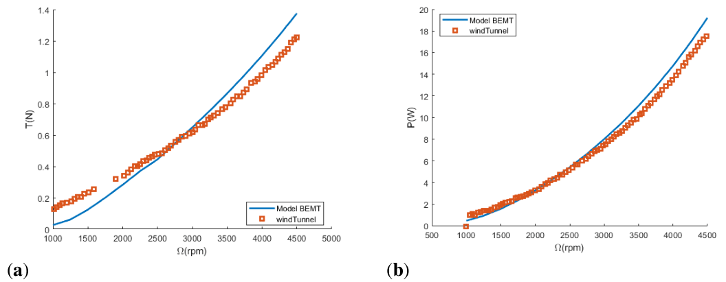
Figure 9 Comparison between model estimations and experimental data from18
(a) Thrust (N) versus rotational speed (Ω) rpm.

  1. b=2
  2. R=0.1775, Rmin=0.0845R.
  3. Ω=1000-4500rpm.
  4. c=0.0225, straight blade.
  5. Linear twist θ_0=11 deg, Δθ=-10.833 deg
  6. Airfoil NACA 0018.

Forward flight validation

Data from17 is used for forward flight model. Since no information about the chord distribution or twist was provided in the document, the data from a T18 rotor was used. Twist and chord distributions of the rotor are available in.19 Figure 10 shows the results.

  1. Mass=2.13 kg
  2. R=0.12m, Rmin=0.1R

Figure 10 Comparison between forward flight model Power (W) estimations versus forward flight speed (Vf(m/s)) and experimental data from.16

Power is underestimated for low velocities, however, as stated during the theoretical explanation, the model can only apply to cases in which ( μ x >0.1) MathType@MTEF@5@5@+= feaagKart1ev2aqatCvAUfeBSjuyZL2yd9gzLbvyNv2CaerbuLwBLn hiov2DGi1BTfMBaeXatLxBI9gBaerbd9wDYLwzYbItLDharqqtubsr 4rNCHbGeaGqk0dg9crFfpeea0xh9v8qiW7rqqrFfpeea0xe9Lq=Jc9 vqaqpepm0xbba9pwe9Q8fs0=yqaqpepae9pg0FirpepeKkFr0xfr=x fr=xb9adbaqaaeGaciGaaiaabeqaamaabaabaaGcbaaeaaaaaaaaa8 qacaGGOaGaeqiVd02damaaBaaaleaapeGaamiEaaWdaeqaaOWdbiab g6da+iaaicdacaGGUaGaaGymaiaacMcaaaa@3FE1@ . Consequently, speed of 10 m/s was set as the minimum speed for optimizations.

Optimization

Among the available optimization methods, PatternSearch was chosen because it can handle robustly smooth and non-smooth problems with all kinds of boundary conditions20 chapter 1.

Total rotor power was set as the objective function. Moreover, four chord and twist distributions were defined. They were combined resulting in 11 optimization cases performed at hovering for a supposed mass of 0.6 kg (1 rotor) and at forward flight for a quadrotor of 2.5 kg at three different advance speeds (10, 15, & 20 m/s). The baseline is a straight untwisted blade rotor with a radius (R) of 20 cm, a chord of 2 cm, and 10 deg pitch. Besides that, the optimization is constrained and bounded for avoiding negative pitch or chord. Additionally, a penalization is used for cases that do not fulfill the limitation μ x 0.1 MathType@MTEF@5@5@+= feaagKart1ev2aqatCvAUfeBSjuyZL2yd9gzLbvyNv2CaerbuLwBLn hiov2DGi1BTfMBaeXatLxBI9gBaerbd9wDYLwzYbItLDharqqtubsr 4rNCHbGeaGqk0dg9crFfpeea0xh9v8qiW7rqqrFfpeea0xe9Lq=Jc9 vqaqpepm0xbba9pwe9Q8fs0=yqaqpepae9pg0FirpepeKkFr0xfr=x fr=xb9adbaqaaeGaciGaaiaabeqaamaabaabaaGcbaaeaaaaaaaaa8 qacqaH8oqBpaWaaSbaaSqaa8qacaWG4baapaqabaGcpeGaeyyzImRa aGimaiaac6cacaaIXaaaaa@3F46@ .

f  μ x <0.1P=P/ μ x MathType@MTEF@5@5@+= feaagKart1ev2aqatCvAUfeBSjuyZL2yd9gzLbvyNv2CaerbuLwBLn hiov2DGi1BTfMBaeXatLxBI9gBaerbd9wDYLwzYbItLDharqqtubsr 4rNCHbGeaGqk0dg9crFfpeea0xh9v8qiW7rqqrFfpeea0xe9Lq=Jc9 vqaqpepm0xbba9pwe9Q8fs0=yqaqpepae9pg0FirpepeKkFr0xfr=x fr=xb9adbaqaaeGaciGaaiaabeqaamaabaabaaGcbaaeaaaaaaaaa8 qacaWGMbGaaiiOaiabeY7aT9aadaWgaaWcbaWdbiaadIhaa8aabeaa k8qacqGH8aapcaaIWaGaaiOlaiaaigdacqGHsgIRcaWGqbGaeyypa0 Jaamiuaiaac+cacqaH8oqBpaWaaSbaaSqaa8qacaWG4baapaqabaaa aa@48F0@ (15)

PatternSearch optimization is divided in 2 steps: mesh creation and polling. The default algorithm is GPS algorithm. It creates 2N searching vectors used for creating additional evaluation points, N is the number of independent optimization variables. Those are director vectors of dimension 1×N:[±1 0...], [0±1...] MathType@MTEF@5@5@+= feaagKart1ev2aqatCvAUfeBSjuyZL2yd9gzLbvyNv2CaerbuLwBLn hiov2DGi1BTfMBaeXatLxBI9gBaerbd9wDYLwzYbItLDharqqtubsr 4rNCHbGeaGqk0dg9crFfpeea0xh9v8qiW7rqqrFfpeea0xe9Lq=Jc9 vqaqpepm0xbba9pwe9Q8fs0=yqaqpepae9pg0FirpepeKkFr0xfr=x fr=xb9adbaqaaeGaciGaaiaabeqaamaabaabaaGcbaaeaaaaaaaaa8 qacaaIXaGaey41aqRaamOtaiaacQdacaGGBbGaeyySaeRaaGymaiaa cckacaaIWaGaaiOlaiaac6cacaGGUaGaaiyxaiaacYcacaGGGcGaai 4waiaaicdacqGHXcqScaaIXaGaaiOlaiaac6cacaGGUaGaaiyxaaaa @4DFF@ etc. The mesh is created using a scalar Δ m MathType@MTEF@5@5@+= feaagKart1ev2aqatCvAUfeBSjuyZL2yd9gzLbvyNv2CaerbuLwBLn hiov2DGi1BTfMBaeXatLxBI9gBaerbd9wDYLwzYbItLDharqqtubsr 4rNCHbGeaGqk0dg9crFfpeea0xh9v8qiW7rqqrFfpeea0xe9Lq=Jc9 vqaqpepm0xbba9pwe9Q8fs0=yqaqpepae9pg0FirpepeKkFr0xfr=x fr=xb9adbaqaaeGaciGaaiaabeqaamaabaabaaGcbaaeaaaaaaaaa8 qacaqGuoWdamaaCaaaleqabaWdbiaab2gaaaaaaa@3A88@ , which is the mesh size of default value 1. The points are created using the initial condition ( x 0 ) MathType@MTEF@5@5@+= feaagKart1ev2aqatCvAUfeBSjuyZL2yd9gzLbvyNv2CaerbuLwBLn hiov2DGi1BTfMBaeXatLxBI9gBaerbd9wDYLwzYbItLDharqqtubsr 4rNCHbGeaGqk0dg9crFfpeea0xh9v8qiW7rqqrFfpeea0xe9Lq=Jc9 vqaqpepm0xbba9pwe9Q8fs0=yqaqpepae9pg0FirpepeKkFr0xfr=x fr=xb9adbaqaaeGaciGaaiaabeqaamaabaabaaGcbaWaaeWaaeaaqa aaaaaaaaWdbiaadIhapaWaaSbaaSqaa8qacaaIWaaapaqabaaakiaa wIcacaGLPaaaaaa@3BD6@ , the mesh size ( Δ m ) MathType@MTEF@5@5@+= feaagKart1ev2aaatCvAUfeBSjuyZL2yd9gzLbvyNv2CaerbuLwBLn hiov2DGi1BTfMBaeXatLxBI9gBaerbd9wDYLwzYbItLDharqqtubsr 4rNCHbGeaGqk0dg9crFfpeea0xh9v8qiW7rqqrFfpeea0xe9Lq=Jc9 vqaqpepm0xbba9pwe9Q8fs0=yqaqpepae9pg0FirpepeKkFr0xfr=x fr=xb9adbaqaaeGaciGaaiaabeqaamaabaabaaGcbaWaaeWaaeaaju gibabaaaaaaaaapeGaeuiLdq0cpaWaaWbaaeqabaqcLbmapeGaamyB aaaaaOWdaiaawIcacaGLPaaaaaa@3E34@ and the searching vectors ( v i ) MathType@MTEF@5@5@+= feaagKart1ev2aqatCvAUfeBSjuyZL2yd9gzLbvyNv2CaerbuLwBLn hiov2DGi1BTfMBaeXatLxBI9gBaerbd9wDYLwzYbItLDharqqtubsr 4rNCHbGeaGqk0dg9crFfpeea0xh9v8qiW7rqqrFfpeea0xe9Lq=Jc9 vqaqpepm0xbba9pwe9Q8fs0=yqaqpepae9pg0FirpepeKkFr0xfr=x fr=xb9adbaqaaeGaciGaaiaabeqaamaabaabaaGcbaWaaeWaaeaaqa aaaaaaaaWdbiaadAhapaWaaSbaaSqaa8qacaWGPbaapaqabaaakiaa wIcacaGLPaaaaaa@3C08@ .

x i = x 0 + Δ m v i MathType@MTEF@5@5@+= feaagKart1ev2aaatCvAUfeBSjuyZL2yd9gzLbvyNv2CaerbuLwBLn hiov2DGi1BTfMBaeXatLxBI9gBaerbd9wDYLwzYbItLDharqqtubsr 4rNCHbGeaGqk0dg9crFfpeea0xh9v8qiW7rqqrFfpeea0xe9Lq=Jc9 vqaqpepm0xbba9pwe9Q8fs0=yqaqpepae9pg0FirpepeKkFr0xfr=x fr=xb9adbaqaaeGaciGaaiaabeqaamaabaabaaGcbaaeaaaaaaaaa8 qacaWG4bWdamaaBaaaleaapeGaamyAaaWdaeqaaOWdbiabg2da9iaa dIhapaWaaSbaaSqaa8qacaaIWaaapaqabaGcpeGaey4kaSscLbsaca qGuoWcpaWaaWbaaeqabaqcLbmapeGaamyBaaaakiaadAhapaWaaSba aSqaa8qacaWGPbaapaqabaaaaa@4505@ (16)

After that, the mesh is evaluated, that is called polling. By default, it evaluates until finding one point with a lower value than the original, successful poll, the new point is selected, and the mesh is expanded. Otherwise, the poll is unsuccessful, and the mesh size is reduced. Expansion and contraction factors are 2 and 0.5. The process is repeated until the stopping criteria is reached.

  1. The mesh size is less than the MeshTolerance (1e-6).
  2. Number of iterations reaches MaxIteration ( 100×N ) MathType@MTEF@5@5@+= feaagKart1ev2aqatCvAUfeBSjuyZL2yd9gzLbvyNv2CaerbuLwBLn hiov2DGi1BTfMBaeXatLxBI9gBaerbd9wDYLwzYbItLDharqqtubsr 4rNCHbGeaGqk0dg9crFfpeea0xh9v8qiW7rqqrFfpeea0xe9Lq=Jc9 vqaqpepm0xbba9pwe9Q8fs0=yqaqpepae9pg0FirpepeKkFr0xfr=x fr=xb9adbaqaaeGaciGaaiaabeqaamaabaabaaGcbaaeaaaaaaaaa8 qadaqadaqaaiaaigdacaaIWaGaaGimaiabgEna0kaad6eaaiaawIca caGLPaaaaaa@3ED4@ .
  3. Maximum number of function evaluations reached ( 2000×N ) MathType@MTEF@5@5@+= feaagKart1ev2aqatCvAUfeBSjuyZL2yd9gzLbvyNv2CaerbuLwBLn hiov2DGi1BTfMBaeXatLxBI9gBaerbd9wDYLwzYbItLDharqqtubsr 4rNCHbGeaGqk0dg9crFfpeea0xh9v8qiW7rqqrFfpeea0xe9Lq=Jc9 vqaqpepm0xbba9pwe9Q8fs0=yqaqpepae9pg0FirpepeKkFr0xfr=x fr=xb9adbaqaaeGaciGaaiaabeqaamaabaabaaGcbaaeaaaaaaaaa8 qadaqadaqaaiaaikdacaaIWaGaaGimaiaaicdacqGHxdaTcaWGobaa caGLOaGaayzkaaaaaa@3F8F@
  4. If after a successful poll, both, distance between initial and new point and mesh size is less than StepTolerance (1e-6).
  5. If after a successful poll the change in the evaluation function is less than StepTolerance (1e-6).

Full information about PatternSearch and how it works can be found in MATLAB PDF documentation20 chapter 6.

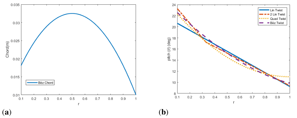
Twist and chord distributions and parameters

  1. Linear twist and Linear chord parameters: root pitch and differential pitch (θ0, slp) and root chord and tip/root chord ratio ( c root ,tap ) MathType@MTEF@5@5@+= feaagKart1ev2aqatCvAUfeBSjuyZL2yd9gzLbvyNv2CaerbuLwBLn hiov2DGi1BTfMBaeXatLxBI9gBaerbd9wDYLwzYbItLDharqqtubsr 4rNCHbGeaGqk0dg9crFfpeea0xh9v8qiW7rqqrFfpeea0xe9Lq=Jc9 vqaqpepm0xbba9pwe9Q8fs0=yqaqpepae9pg0FirpepeKkFr0xfr=x fr=xb9adbaqaaeGaciGaaiaabeqaamaabaabaaGcbaWaaeWaaeaaqa aaaaaaaaWdbiaadogapaWaaSbaaSqaa8qacaWGYbGaam4Baiaad+ga caWG0baapaqabaGccaGGSaGaamiDaiaadggacaWGWbaacaGLOaGaay zkaaaaaa@4263@ .

θ( r )= θ 0 +slpr c( r )= c root ( 1+r( tap1 ) ) MathType@MTEF@5@5@+= feaagKart1ev2aqatCvAUfeBSjuyZL2yd9gzLbvyNv2CaerbuLwBLn hiov2DGi1BTfMBaeXatLxBI9gBaerbd9wDYLwzYbItLDharqqtubsr 4rNCHbGeaGqk0dg9crFfpeea0xh9v8qiW7rqqrFfpeea0xe9Lq=Jc9 vqaqpepm0xbba9pwe9Q8fs0=yqaqpepae9pg0FirpepeKkFr0xfr=x fr=xb9adbaqaaeGaciGaaiaabeqaamaabaabaaGceaqabeaaqaaaaa aaaaWdbiabeI7aXnaabmaapaqaa8qacaWGYbaacaGLOaGaayzkaaGa eyypa0JaeqiUde3damaaBaaaleaapeGaaGimaaWdaeqaaOWdbiabgU caRiaadohacaWGSbGaamiCaiabgwSixlaadkhaaeaacaWGJbWaaeWa a8aabaWdbiaadkhaaiaawIcacaGLPaaacqGH9aqpcaWGJbWdamaaBa aaleaapeGaamOCaiaad+gacaWGVbGaamiDaaWdaeqaaOWdbmaabmaa paqaa8qacaaIXaGaey4kaSIaamOCamaabmaapaqaa8qacaWG0bGaam yyaiaadchacqGHsislcaaIXaaacaGLOaGaayzkaaaacaGLOaGaayzk aaaaaaa@5B9A@ (17)

  1. 2 Linear twist and Linear chord parameters: (θ0, slp1, slp2, rper1) and ( c root ,tap1, tap2, rper2 ) MathType@MTEF@5@5@+= feaagKart1ev2aqatCvAUfeBSjuyZL2yd9gzLbvyNv2CaerbuLwBLn hiov2DGi1BTfMBaeXatLxBI9gBaerbd9wDYLwzYbItLDharqqtubsr 4rNCHbGeaGqk0dg9crFfpeea0xh9v8qiW7rqqrFfpeea0xe9Lq=Jc9 vqaqpepm0xbba9pwe9Q8fs0=yqaqpepae9pg0FirpepeKkFr0xfr=x fr=xb9adbaqaaeGaciGaaiaabeqaamaabaabaaGcbaWaaeWaaeaaqa aaaaaaaaWdbiaadogapaWaaSbaaSqaa8qacaWGYbGaam4Baiaad+ga caWG0baapaqabaGccaGGSaWdbiaadshacaWGHbGaamiCaiaaigdaca GGSaGaaeiiaiaadshacaWGHbGaamiCaiaaikdacaGGSaGaaeiiaiaa dkhacaWGWbGaamyzaiaadkhacaaIYaaapaGaayjkaiaawMcaaaaa@4DFC@ . Where is the blade section where segment changes.

θ ( r ) 1 = θ 0 + slp1 r perc1 r,   θ ( r ) 2 =θ ( r perc1 ) 1 + slp2 1 r perc1 ( r r perc1 ) c ( r ) 1 = c root ( 1+r( tap1 ) ),   c ( r ) 2 =c ( r perc2 ) 1 ( 1+ tap21 1 r perc2 ( r r perc2 ) ) MathType@MTEF@5@5@+= feaagKart1ev2aqatCvAUfeBSjuyZL2yd9gzLbvyNv2CaerbuLwBLn hiov2DGi1BTfMBaeXatLxBI9gBaerbd9wDYLwzYbItLDharqqtubsr 4rNCHbGeaGqk0dg9crFfpeea0xh9v8qiW7rqqrFfpeea0xe9Lq=Jc9 vqaqpepm0xbba9pwe9Q8fs0=yqaqpepae9pg0FirpepeKkFr0xfr=x fr=xb9adbaqaaeGaciGaaiaabeqaamaabaabaaGceaqabeaaqaaaaa aaaaWdbiabeI7aXnaabmaapaqaa8qacaWGYbaacaGLOaGaayzkaaWd amaaBaaaleaapeGaaGymaaWdaeqaaOWdbiabg2da9iabeI7aX9aada WgaaWcbaWdbiaaicdaa8aabeaak8qacqGHRaWkdaWcaaWdaeaapeGa am4CaiaadYgacaWGWbGaaGymaaWdaeaapeGaamOCa8aadaWgaaWcba WdbiaadchacaWGLbGaamOCaiaadogacaaIXaaapaqabaaaaOWdbiab gwSixlaadkhacaGGSaGaaiiOaiaacckacaGGGcGaeqiUde3aaeWaa8 aabaWdbiaadkhaaiaawIcacaGLPaaapaWaaSbaaSqaa8qacaaIYaaa paqabaGcpeGaeyypa0JaeqiUde3aaeWaa8aabaWdbiaadkhapaWaaS baaSqaa8qacaWGWbGaamyzaiaadkhacaWGJbGaaGymaaWdaeqaaaGc peGaayjkaiaawMcaa8aadaWgaaWcbaWdbiaaigdaa8aabeaak8qacq GHRaWkdaWcaaWdaeaapeGaam4CaiaadYgacaWGWbGaaGOmaaWdaeaa peGaaGymaiabgkHiTiaadkhapaWaaSbaaSqaa8qacaWGWbGaamyzai aadkhacaWGJbGaaGymaaWdaeqaaaaak8qadaqadaWdaeaapeGaamOC aiabgkHiTiaadkhapaWaaSbaaSqaa8qacaWGWbGaamyzaiaadkhaca WGJbGaaGymaaWdaeqaaaGcpeGaayjkaiaawMcaaaqaaiaadogadaqa daWdaeaapeGaamOCaaGaayjkaiaawMcaa8aadaWgaaWcbaWdbiaaig daa8aabeaak8qacqGH9aqpcaWGJbWdamaaBaaaleaapeGaamOCaiaa d+gacaWGVbGaamiDaaWdaeqaaOWdbmaabmaapaqaa8qacaaIXaGaey 4kaSIaamOCamaabmaapaqaa8qacaWG0bGaamyyaiaadchacqGHsisl caaIXaaacaGLOaGaayzkaaaacaGLOaGaayzkaaGaaiilaiaacckaca GGGcGaaiiOaiaadogadaqadaWdaeaapeGaamOCaaGaayjkaiaawMca a8aadaWgaaWcbaWdbiaaikdaa8aabeaak8qacqGH9aqpcaWGJbWaae Waa8aabaWdbiaadkhapaWaaSbaaSqaa8qacaWGWbGaamyzaiaadkha caWGJbGaaGOmaaWdaeqaaaGcpeGaayjkaiaawMcaa8aadaWgaaWcba Wdbiaaigdaa8aabeaak8qadaqadaWdaeaapeGaaGymaiabgUcaRmaa laaapaqaa8qacaWG0bGaamyyaiaadchacaaIYaGaeyOeI0IaaGymaa WdaeaapeGaaGymaiabgkHiTiaadkhapaWaaSbaaSqaa8qacaWGWbGa amyzaiaadkhacaWGJbGaaGOmaaWdaeqaaaaak8qadaqadaWdaeaape GaamOCaiabgkHiTiaadkhapaWaaSbaaSqaa8qacaWGWbGaamyzaiaa dkhacaWGJbGaaGOmaaWdaeqaaaGcpeGaayjkaiaawMcaaaGaayjkai aawMcaaaaaaa@BD09@ (18)

  1. Quadratic twist and chord parameters: ( θ 0 , c root , a 1 ,  a 2 ) MathType@MTEF@5@5@+= feaagKart1ev2aaatCvAUfeBSjuyZL2yd9gzLbvyNv2CaerbuLwBLn hiov2DGi1BTfMBaeXatLxBI9gBaerbd9wDYLwzYbItLDharqqtubsr 4rNCHbGeaGqk0dg9crFfpeea0xh9v8qiW7rqqrFfpeea0xe9Lq=Jc9 vqaqpepm0xbba9pwe9Q8fs0=yqaqpepae9pg0FirpepeKkFr0xfr=x fr=xb9adbaqaaeGaciGaaiaabeqaamaabaabaaGcbaWaaeWaaeaaqa aaaaaaaaWdbiabeI7aX9aadaWgaaWcbaWdbiaaicdaa8aabeaakiaa cYcapeGaam4ya8aadaWgaaWcbaWdbiaadkhacaWGVbGaam4Baiaads haa8aabeaakiaacYcapeGaamyya8aadaWgaaWcbaWdbiaaigdaa8aa beaak8qacaGGSaGaaiiOaiaadggapaWaaSbaaSqaa8qacaaIYaaapa qabaaakiaawIcacaGLPaaaaaa@4921@ , (a) parameters control the chord/pitch at the tip.

θ( r )= θ 0 + a 1 r 2 2 a 1 r  c( r )= c root ( 1+ a 2 r 2 2 a 2 r ) MathType@MTEF@5@5@+= feaagKart1ev2aqatCvAUfeBSjuyZL2yd9gzLbvyNv2CaerbuLwBLn hiov2DGi1BTfMBaeXatLxBI9gBaerbd9wDYLwzYbItLDharqqtubsr 4rNCHbGeaGqk0dg9crFfpeea0xh9v8qiW7rqqrFfpeea0xe9Lq=Jc9 vqaqpepm0xbba9pwe9Q8fs0=yqaqpepae9pg0FirpepeKkFr0xfr=x fr=xb9adbaqaaeGaciGaaiaabeqaamaabaabaaGceaqabeaaqaaaaa aaaaWdbiabeI7aXnaabmaapaqaa8qacaWGYbaacaGLOaGaayzkaaGa eyypa0JaeqiUde3damaaBaaaleaapeGaaGimaaWdaeqaaOWdbiabgU caRiaadggapaWaaSbaaSqaa8qacaaIXaaapaqabaGcpeGaeyyXICTa amOCa8aadaahaaWcbeqaa8qacaaIYaaaaOGaeyOeI0IaaGOmaiaadg gapaWaaSbaaSqaa8qacaaIXaaapaqabaGcpeGaeyyXICTaamOCaaqa aiaacckacaWGJbWaaeWaa8aabaWdbiaadkhaaiaawIcacaGLPaaacq GH9aqpcaWGJbWdamaaBaaaleaapeGaamOCaiaad+gacaWGVbGaamiD aaWdaeqaaOWdbmaabmaapaqaa8qacaaIXaGaey4kaSIaamyya8aada WgaaWcbaWdbiaaikdaa8aabeaak8qacqGHflY1caWGYbWdamaaCaaa leqabaWdbiaaikdaaaGccqGHsislcaaIYaGaamyya8aadaWgaaWcba Wdbiaaikdaa8aabeaak8qacqGHflY1caWGYbaacaGLOaGaayzkaaaa aaa@6A54@ (19)

  1. Cubic Bezier twist parameters: (θ0, θtip, r3, y4, r5, y6)→P0(0, θ0), P2(1, θtip), P1(r3, y4), P3(r5, y6), the parameters ( r,y ) MathType@MTEF@5@5@+= feaagKart1ev2aqatCvAUfeBSjuyZL2yd9gzLbvyNv2CaerbuLwBLn hiov2DGi1BTfMBaeXatLxBI9gBaerbd9wDYLwzYbItLDharqqtubsr 4rNCHbGeaGqk0dg9crFfpeea0xh9v8qiW7rqqrFfpeea0xe9Lq=Jc9 vqaqpepm0xbba9pwe9Q8fs0=yqaqpepae9pg0FirpepeKkFr0xfr=x fr=xb9adbaqaaeGaciGaaiaabeqaamaabaabaaGcbaaeaaaaaaaaa8 qadaqadaWdaeaapeGaamOCaiaacYcacaWG5baacaGLOaGaayzkaaaa aa@3C7F@ are the coordinates of the spline points.

θ( r )= ( 1r ) 3 P0+3 ( 1r ) 2 rP1+3( 1r ) r 2 P2+ r 3 P3 MathType@MTEF@5@5@+= feaagKart1ev2aqatCvAUfeBSjuyZL2yd9gzLbvyNv2CaerbuLwBLn hiov2DGi1BTfMBaeXatLxBI9gBaerbd9wDYLwzYbItLDharqqtubsr 4rNCHbGeaGqk0dg9crFfpeea0xh9v8qiW7rqqrFfpeea0xe9Lq=Jc9 vqaqpepm0xbba9pwe9Q8fs0=yqaqpepae9pg0FirpepeKkFr0xfr=x fr=xb9adbaqaaeGaciGaaiaabeqaamaabaabaaGcbaaeaaaaaaaaa8 qacqaH4oqCdaqadaWdaeaapeGaamOCaaGaayjkaiaawMcaaiabg2da 9maabmaapaqaa8qacaaIXaGaeyOeI0IaamOCaaGaayjkaiaawMcaa8 aadaahaaWcbeqaa8qacaaIZaaaaOGaamiuaiaaicdacqGHRaWkcaaI ZaWaaeWaa8aabaWdbiaaigdacqGHsislcaWGYbaacaGLOaGaayzkaa WdamaaCaaaleqabaWdbiaaikdaaaGccaWGYbGaeyyXICTaamiuaiaa igdacqGHRaWkcaaIZaWaaeWaa8aabaWdbiaaigdacqGHsislcaWGYb aacaGLOaGaayzkaaGaamOCa8aadaahaaWcbeqaa8qacaaIYaaaaOGa eyyXICTaamiuaiaaikdacqGHRaWkcaWGYbWdamaaCaaaleqabaWdbi aaiodaaaGccaWGqbGaaG4maaaa@6087@ (20)

  1. Cubic Bezier chord parameters: ( c root ,tap, r3,y4,r5,y6 )P0( 0, c root ),P2( 1,tap· c root ),P1(r3, y4), P3(r5, y6) MathType@MTEF@5@5@+= feaagKart1ev2aaatCvAUfeBSjuyZL2yd9gzLbvyNv2CaerbuLwBLn hiov2DGi1BTfMBaeXatLxBI9gBaerbd9wDYLwzYbItLDharqqtubsr 4rNCHbGeaGqk0dg9crFfpeea0xh9v8qiW7rqqrFfpeea0xe9Lq=Jc9 vqaqpepm0xbba9pwe9Q8fs0=yqaqpepae9pg0FirpepeKkFr0xfr=x fr=xb9adbaqaaeGaciGaaiaabeqaamaabaabaaGcbaWaaeWaaeaaqa aaaaaaaaWdbiaadogapaWaaSbaaSqaa8qacaWGYbGaam4Baiaad+ga caWG0baapaqabaGccaGGSaWdbiaadshacaWGHbGaamiCaiaacYcaca qGGaGaamOCaiaaiodacaGGSaGaamyEaiaaisdacaGGSaGaamOCaiaa iwdacaGGSaGaamyEaiaaiAdaa8aacaGLOaGaayzkaaWdbiabgkziUk aadcfacaaIWaWaaeWaaeaacaaIWaGaaiilaiaadogapaWaaSbaaSqa a8qacaWGYbGaam4Baiaad+gacaWG0baapaqabaaak8qacaGLOaGaay zkaaGaaiilaiaadcfacaaIYaWaaeWaaeaacaaIXaGaaiilaiaadsha caWGHbGaamiCaiaacElacaWGJbWdamaaBaaaleaapeGaamOCaiaad+ gacaWGVbGaamiDaaWdaeqaaaGcpeGaayjkaiaawMcaaiaacYcacaWG qbGaaGyma8aacaGGOaWdbiaadkhacaaIZaGaaiilaiaabccacaWG5b GaaGina8aacaGGPaWdbiaacYcacaqGGaGaamiuaiaaiodapaGaaiik a8qacaWGYbGaaGynaiaacYcacaqGGaGaamyEaiaaiAdapaGaaiykaa aa@78C0@

c( r )= ( 1r ) 3 P0+3 ( 1r ) 2 rP1+3( 1r ) r 2 P2+ r 3 P3 MathType@MTEF@5@5@+= feaagKart1ev2aaatCvAUfeBSjuyZL2yd9gzLbvyNv2CaerbuLwBLn hiov2DGi1BTfMBaeXatLxBI9gBaerbd9wDYLwzYbItLDharqqtubsr 4rNCHbGeaGqk0dg9crFfpeea0xh9v8qiW7rqqrFfpeea0xe9Lq=Jc9 vqaqpepm0xbba9pwe9Q8fs0=yqaqpepae9pg0FirpepeKkFr0xfr=x fr=xb9adbaqaaeGaciGaaiaabeqaamaabaabaaGcbaaeaaaaaaaaa8 qacaWGJbWaaeWaa8aabaWdbiaadkhaaiaawIcacaGLPaaacqGH9aqp daqadaWdaeaapeGaaGymaiabgkHiTiaadkhaaiaawIcacaGLPaaapa WaaWbaaSqabeaapeGaaG4maaaakiaadcfacaaIWaGaey4kaSIaaG4m amaabmaapaqaa8qacaaIXaGaeyOeI0IaamOCaaGaayjkaiaawMcaa8 aadaahaaWcbeqaa8qacaaIYaaaaOGaamOCaiabgwSixlaadcfacaaI XaGaey4kaSIaaG4mamaabmaapaqaa8qacaaIXaGaeyOeI0IaamOCaa GaayjkaiaawMcaaiaadkhapaWaaWbaaSqabeaapeGaaGOmaaaakiab gwSixlaadcfacaaIYaGaey4kaSIaamOCa8aadaahaaWcbeqaa8qaca aIZaaaaOGaamiuaiaaiodaaaa@5FB8@ (21)

The bounds of the optimization variables are gathered in Tables 1 & 2. Where R is the radius of the rotor (20cm).

Bound

Croot(m)

tap

tap1

tap2

a2

rper1

r3

r4

y3(m)

y4(m)

Low


0.2

0.2

0.7

0

0.2

0.2

0.55


Upper


1.3

1.3

1

1

0.8

0.45

0.8


Table 1 Chord optimization parameters’ bounds

Bound

θroot(deg)

slp(deg)

slp1(deg)

slp2(deg)

a1(deg)

rper2

r3

r4

y3(deg)

y4(deg)

Low

5

-35

-35

-35

0

0.1

0.2

0.55

-45

-45

Upper

35

0

0

0

25

0.9

0.45

0.8

45

45

Table 2 Twist optimization parameters’ bounds

Additionally, the problem is constrained for avoiding negative pitch using inequalities.

  1. Linear distribution: |Slp|-θ_root≤0
  2. Quadratic distribution: a_1-θ_root≤0
  3. 2. Linear distribution: |slp1+slp2|-θ_root≤0
  4. Bézier distribution: θ( r )0r[ 0,1 ] MathType@MTEF@5@5@+= feaagKart1ev2aaatCvAUfeBSjuyZL2yd9gzLbvyNv2CaerbuLwBLn hiov2DGi1BTfMBaeXatLxBI9gBaerbd9wDYLwzYbItLDharqqtubsr 4rNCHbGeaGqk0dg9crFfpeea0xh9v8qiW7rqqrFfpeea0xe9Lq=Jc9 vqaqpepm0xbba9pwe9Q8fs0=yqaqpepae9pg0FirpepeKkFr0xfr=x fr=xb9adbaqaaeGaciGaaiaabeqaamaabaabaaGcbaqcLbsaqaaaaa aaaaWdbiabgkHiTiabeI7aXPWdamaabmaabaqcLbsapeGaamOCaaGc paGaayjkaiaawMcaaKqzGeWdbiabgsMiJkaaicdacqGHaiIicaWGYb GaeyicI4ScpaWaamWaaeaajugib8qacaaIWaGaaiilaiaaigdaaOWd aiaawUfacaGLDbaaaaa@49F5@

PatternSearch verifies that the points of the mesh fulfill the limits. If not, they are projected in the feasible subspace. The case of Bézier distribution limitation is more complex, nonlinear constraints problems are solved using Augmented Lagrangian Pattern Search (ALPS) algorithm, which solves several subproblems. ALPS algorithm combines penalization methods, who transforms a constrained problem into a non-constrained problem adding a penalization term, and lagrange methods for solving subproblems and reaching the optimal solution. This can be used for equality constraints and inequality constraints. The combination of both avoids problems with the penalization going to infinity for ensuring convergence. The general expression for the constrained subproblem with equalities ( ce q i ) MathType@MTEF@5@5@+= feaagKart1ev2aqatCvAUfeBSjuyZL2yd9gzLbvyNv2CaerbuLwBLn hiov2DGi1BTfMBaeXatLxBI9gBaerbd9wDYLwzYbItLDharqqtubsr 4rNCHbGeaGqk0dg9crFfpeea0xh9v8qiW7rqqrFfpeea0xe9Lq=Jc9 vqaqpepm0xbba9pwe9Q8fs0=yqaqpepae9pg0FirpepeKkFr0xfr=x fr=xb9adbaqaaeGaciGaaiaabeqaamaabaabaaGcbaWaaeWaaeaaqa aaaaaaaaWdbiaadogacaWGLbGaamyCa8aadaWgaaWcbaWdbiaadMga a8aabeaaaOGaayjkaiaawMcaaaaa@3DD5@ , inequalities ( c i ) MathType@MTEF@5@5@+= feaagKart1ev2aqatCvAUfeBSjuyZL2yd9gzLbvyNv2CaerbuLwBLn hiov2DGi1BTfMBaeXatLxBI9gBaerbd9wDYLwzYbItLDharqqtubsr 4rNCHbGeaGqk0dg9crFfpeea0xh9v8qiW7rqqrFfpeea0xe9Lq=Jc9 vqaqpepm0xbba9pwe9Q8fs0=yqaqpepae9pg0FirpepeKkFr0xfr=x fr=xb9adbaqaaeGaciGaaiaabeqaamaabaabaaGcbaWaaeWaaeaaqa aaaaaaaaWdbiaadogapaWaaSbaaSqaa8qacaWGPbaapaqabaaakiaa wIcacaGLPaaaaaa@3BF5@ and penalization factor (ρ) is:

Θ( x, λ, s, ρ )=f( x ) i=1 m Λ i s i log( s i c i ( x ) )+  i=m+1 mt Λ i ce q i ( x ) + ρ 2 i=m+1 mt ce q i ( x ) 2 MathType@MTEF@5@5@+= feaagKart1ev2aaatCvAUfeBSjuyZL2yd9gzLbvyNv2CaerbuLwBLn hiov2DGi1BTfMBaeXatLxBI9gBaerbd9wDYLwzYbItLDharqqtubsr 4rNCHbGeaGqk0dg9crFfpeea0xh9v8qiW7rqqrFfpeea0xe9Lq=Jc9 vqaqpepm0xbba9pwe9Q8fs0=yqaqpepae9pg0FirpepeKkFr0xfr=x fr=xb9adbaqaaeGaciGaaiaabeqaamaabaabaaGceaqabeaaqaaaaa aaaaWdbiaabI5adaqadaWdaeaapeGaaeiEaiaacYcacaqGGcGaae4U diaacYcacaqGGcGaae4CaiaacYcacaqGGcGaaeyWdaGaayjkaiaawM caaiabg2da9iaadAgadaqadaWdaeaapeGaamiEaaGaayjkaiaawMca aiabgkHiTmaawahabeWcpaqaa8qacaWGPbGaeyypa0JaaGymaaWdae aapeGaamyBaaqdpaqaa8qacqGHris5aaGccaqGBoWdamaaBaaaleaa peGaamyAaaWdaeqaaOWdbiaadohapaWaaSbaaSqaa8qacaWGPbaapa qabaGcpeGaciiBaiaac+gacaGGNbWaaeWaa8aabaWdbiaadohapaWa aSbaaSqaa8qacaWGPbaapaqabaGcpeGaeyOeI0Iaam4ya8aadaWgaa WcbaWdbiaadMgaa8aabeaak8qadaqadaWdaeaapeGaamiEaaGaayjk aiaawMcaaaGaayjkaiaawMcaaiabgUcaRiaacckadaGfWbqabSWdae aapeGaamyAaiabg2da9iaad2gacqGHRaWkcaaIXaaapaqaa8qacaWG TbGaamiDaaqdpaqaa8qacqGHris5aaGccaqGBoWdamaaBaaaleaape GaamyAaaWdaeqaaOWdbiaadogacaWGLbGaamyCa8aadaWgaaWcbaWd biaadMgaa8aabeaak8qadaqadaWdaeaapeGaamiEaaGaayjkaiaawM caaaqaaiabgUcaRmaalaaapaqaa8qacqaHbpGCa8aabaWdbiaaikda aaWaaybCaeqal8aabaWdbiaadMgacqGH9aqpcaWGTbGaey4kaSIaaG ymaaWdaeaapeGaamyBaiaadshaa0WdaeaapeGaeyyeIuoaaOGaam4y aiaadwgacaWGXbWdamaaBaaaleaapeGaamyAaaWdaeqaaOWdbmaabm aapaqaa8qacaWG4baacaGLOaGaayzkaaWdamaaCaaaleqabaWdbiaa ikdaaaaaaaa@8B69@ (22)

The previous expression is the Lagrangian function of a constrained optimization problem with the addition of the penalization factor for the equality constraints. This subproblem is handled separately from upper and lower bounds and if required, linear constrains, which can be handled by projection of the points in the limits and subspaces. The subproblem expression considers the inequalities assuming the equivalence of the constraints ( c i 0 ) MathType@MTEF@5@5@+= feaagKart1ev2aqatCvAUfeBSjuyZL2yd9gzLbvyNv2CaerbuLwBLn hiov2DGi1BTfMBaeXatLxBI9gBaerbd9wDYLwzYbItLDharqqtubsr 4rNCHbGeaGqk0dg9crFfpeea0xh9v8qiW7rqqrFfpeea0xe9Lq=Jc9 vqaqpepm0xbba9pwe9Q8fs0=yqaqpepae9pg0FirpepeKkFr0xfr=x fr=xb9adbaqaaeGaciGaaiaabeqaamaabaabaaGcbaaeaaaaaaaaa8 qadaqadaqaaiaadogapaWaaSbaaSqaa8qacaWGPbaapaqabaGcpeGa eyizImQaaGimaaGaayjkaiaawMcaaaaa@3E74@ and ( s i log( s i c i ( x ) ) ) MathType@MTEF@5@5@+= feaagKart1ev2aqatCvAUfeBSjuyZL2yd9gzLbvyNv2CaerbuLwBLn hiov2DGi1BTfMBaeXatLxBI9gBaerbd9wDYLwzYbItLDharqqtubsr 4rNCHbGeaGqk0dg9crFfpeea0xh9v8qiW7rqqrFfpeea0xe9Lq=Jc9 vqaqpepm0xbba9pwe9Q8fs0=yqaqpepae9pg0FirpepeKkFr0xfr=x fr=xb9adbaqaaeGaciGaaiaabeqaamaabaabaaGcbaaeaaaaaaaaa8 qadaqadaqaaiaadohapaWaaSbaaSqaa8qacaWGPbaapaqabaGcpeGa ciiBaiaac+gacaGGNbWaaeWaa8aabaWdbiaadohapaWaaSbaaSqaa8 qacaWGPbaapaqabaGcpeGaeyOeI0Iaam4ya8aadaWgaaWcbaWdbiaa dMgaa8aabeaak8qadaqadaWdaeaapeGaamiEaaGaayjkaiaawMcaaa GaayjkaiaawMcaaaGaayjkaiaawMcaaaaa@48C3@ where s i MathType@MTEF@5@5@+= feaagKart1ev2aqatCvAUfeBSjuyZL2yd9gzLbvyNv2CaerbuLwBLn hiov2DGi1BTfMBaeXatLxBI9gBaerbd9wDYLwzYbItLDharqqtubsr 4rNCHbGeaGqk0dg9crFfpeea0xh9v8qiW7rqqrFfpeea0xe9Lq=Jc9 vqaqpepm0xbba9pwe9Q8fs0=yqaqpepae9pg0FirpepeKkFr0xfr=x fr=xb9adbaqaaeGaciGaaiaabeqaamaabaabaaGcbaaeaaaaaaaaa8 qacaWGZbWdamaaBaaaleaapeGaamyAaaWdaeqaaaaa@3A72@ are positive values known as shifts which are computed considering the penalty values (ρ) and the Lagrange multipliers estimates ( Λ i ) MathType@MTEF@5@5@+= feaagKart1ev2aqatCvAUfeBSjuyZL2yd9gzLbvyNv2CaerbuLwBLn hiov2DGi1BTfMBaeXatLxBI9gBaerbd9wDYLwzYbItLDharqqtubsr 4rNCHbGeaGqk0dg9crFfpeea0xh9v8qiW7rqqrFfpeea0xe9Lq=Jc9 vqaqpepm0xbba9pwe9Q8fs0=yqaqpepae9pg0FirpepeKkFr0xfr=x fr=xb9adbaqaaeGaciGaaiaabeqaamaabaabaaGcbaaeaaaaaaaaa8 qadaqadaWdaeaajugib8qacaqGBoWcpaWaaSbaaeaajugWa8qacaqG Pbaal8aabeaaaOWdbiaawIcacaGLPaaaaaa@3E23@ . Moreover, this previous term ensures that the constraint inequality is fulfilled. As a global overview, what the inner algorithm responsible of solving the subproblem seeks is the convergence in a set of values ( x k ) MathType@MTEF@5@5@+= feaagKart1ev2aqatCvAUfeBSjuyZL2yd9gzLbvyNv2CaerbuLwBLn hiov2DGi1BTfMBaeXatLxBI9gBaerbd9wDYLwzYbItLDharqqtubsr 4rNCHbGeaGqk0dg9crFfpeea0xh9v8qiW7rqqrFfpeea0xe9Lq=Jc9 vqaqpepm0xbba9pwe9Q8fs0=yqaqpepae9pg0FirpepeKkFr0xfr=x fr=xb9adbaqaaeGaciGaaiaabeqaamaabaabaaGcbaaeaaaaaaaaa8 qadaqadaWdaeaapeGaamiEa8aadaWgaaWcbaWdbiaadUgaa8aabeaa aOWdbiaawIcacaGLPaaaaaa@3C3B@ that are first-order stationary points, or what is the same, a Kuhn-Tucker points. The algorithm is driven by the penalty factor, which is also used for estimating the Lagrange multipliers and convergence is reached if ( 1 ρ ) MathType@MTEF@5@5@+= feaagKart1ev2aaatCvAUfeBSjuyZL2yd9gzLbvyNv2CaerbuLwBLn hiov2DGi1BTfMBaeXatLxBI9gBaerbd9wDYLwzYbItLDharqqtubsr 4rNCHbGeaGqk0dg9crFfpeea0xh9v8qiW7rqqrFfpeea0xe9Lq=Jc9 vqaqpepm0xbba9pwe9Q8fs0=yqaqpepae9pg0FirpepeKkFr0xfr=x fr=xb9adbaqaaeGaciGaaiaabeqaamaabaabaaGcbaaeaaaaaaaaa8 qadaqadaWdaeaapeWaaSGaaeaacaaIXaaabaGaeqyWdihaaaGaayjk aiaawMcaaaaa@3C66@ tends to a sufficiently small value. For deep details about the algorithm and the inequality constrained it is suggested to check MATLAB user guide documentation20 as well as the article dedicated to Augmented Lagrangian Optimization with inequality constraints and bounds.21

Optimization results and CFD simulations

Hovering optimization

Chord optimization, constant pitch of 10 deg: Tapered blades and quadratic chord distributions did not improve rotor efficiency in these regimes. Straight blade geometry was the optimal. Improving efficiency is represented by the term ( ΔP=100( P opt P BL )/ P BL ) MathType@MTEF@5@5@+= feaagKart1ev2aqatCvAUfeBSjuyZL2yd9gzLbvyNv2CaerbuLwBLn hiov2DGi1BTfMBaeXatLxBI9gBaerbd9wDYLwzYbItLDharqqtubsr 4rNCHbGeaGqk0dg9crFfpeea0xh9v8qiW7rqqrFfpeea0xe9Lq=Jc9 vqaqpepm0xbba9pwe9Q8fs0=yqaqpepae9pg0FirpepeKkFr0xfr=x fr=xb9adbaqaaeGaciGaaiaabeqaamaabaabaaGcbaaeaaaaaaaaa8 qadaqadaWdaeaajugib8qacqqHuoarkiaadcfacqGH9aqpcaaIXaGa aGimaiaaicdacqGHflY1caGGOaGaamiua8aadaWgaaWcbaWdbiaad+ gacaWGWbGaamiDaaWdaeqaaOWdbiabgkHiTiaadcfapaWaaSbaaSqa a8qacaWGcbGaamitaaWdaeqaaaGcpeGaayjkaiaawMcaaiaac+caca WGqbWdamaaBaaaleaapeGaamOqaiaadYeaa8aabeaak8qacaGGPaaa aa@4F13@ , which is the percentual power reduction (-) or increment (+) with respect to the baseline rotor. Regarding to the distribution with two linear segments showed that hexagonal blade platforms can be an interesting alternative to straight blades. Finally, the spline distribution showed similar behavior to the previous distribution. The platform area is increased, and a slight taper is set near the tips, where speeds and profile drag are higher. Optimal parameters are in Table 3 whereas rotor’s comparative is found in Table 4.

Case

Croot(m)

tap / tap2 / a2

rperc

r3 / y4

r5 / y6

1.Linear Chord

0.02

1 / - / -

-

- / -

- / -

Quadratic Chord

0.02

- / - / 0

-

- / -

- / -

2.Linear Chord

0.02

1.3 / 0.6429 / -

0.63

- / -

- / -

Bézier. Chord

0.02

0.8822 / - / -

-

0.409 / 0.04

0.7537 / 0.0261

Table 3 Chord optimal distributions for hovering: 1 Linear segment, quadratic case, 2 linear segment and Bézier distribution
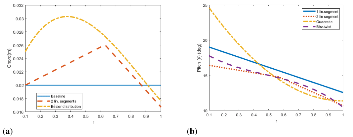
 

Base Line

1.Linear Chord

Quadratic Chord

2.Linear Chord

Bézier Chord

Ω( rad/s ) MathType@MTEF@5@5@+= feaagKart1ev2aaatCvAUfeBSjuyZL2yd9gzLbvyNv2CaerbuLwBLn hiov2DGi1BTfMBaeXatLxBI9gBaerbd9wDYLwzYbItLDharqqtubsr 4rNCHbGeaGqk0dg9crFfpeea0xh9v8qiW7rqqrFfpeea0xe9Lq=Jc9 vqaqpepm0xbba9pwe9Q8fs0=yqaqpepae9pg0FirpepeKkFr0xfr=x fr=xb9adbaqaaeGaciGaaiaabeqaamaabaabaaGcbaqcLbsaqaaaaa aaaaWdbiaabM6ak8aadaqadaqaaKqzGeWdbiaabkhacaqGHbGaaeiz aiaab+cacaqGZbaak8aacaGLOaGaayzkaaaaaa@40B1@

421.74

421.74

421.74

405.28

400.41

Power (W)

52.64

52.64

52.64

50.8085

50.5681

ΔP( % ) MathType@MTEF@5@5@+= feaagKart1ev2aaatCvAUfeBSjuyZL2yd9gzLbvyNv2CaerbuLwBLn hiov2DGi1BTfMBaeXatLxBI9gBaerbd9wDYLwzYbItLDharqqtubsr 4rNCHbGeaGqk0dg9crFfpeea0xh9v8qiW7rqqrFfpeea0xe9Lq=Jc9 vqaqpepm0xbba9pwe9Q8fs0=yqaqpepae9pg0FirpepeKkFr0xfr=x fr=xb9adbaqaaeGaciGaaiaabeqaamaabaabaaGcbaqcLbsaqaaaaa aaaaWdbiaabs5acaqGqbGcpaWaaeWaaeaajugib8qacaqGLaaak8aa caGLOaGaayzkaaaaaa@3DAF@

-

0

0

-3.5

-3.93

Table 4 Performance comparative for hovering of optimized chord cases

Twist optimization, constant chord of 0.02 m:

Moving on to twist optimizations, the model predicts greater improvements for twisted blades. Additionally, the average blade pitch has been increased from the original pitch of 10 deg. This increment reduces the required rotational speed, thereby the profile drag. Furthermore, all distributions, except for the quadratic distribution, which is conditioned by its curve shape, show similar behavior, and have a comparable differential pitch between the root and tip. Like for large-scale rotors, twist optimal rate is negative. Parameters for each distribution and performance results are found in Tables 5 & 6, and they are plotted in Figure 11.


Base Line

1.Linear Twist

Quadratic Twist

2.Linear Twist

Bézier Twist

Ω( rad/s ) MathType@MTEF@5@5@+= feaagKart1ev2aaatCvAUfeBSjuyZL2yd9gzLbvyNv2CaerbuLwBLn hiov2DGi1BTfMBaeXatLxBI9gBaerbd9wDYLwzYbItLDharqqtubsr 4rNCHbGeaGqk0dg9crFfpeea0xh9v8qiW7rqqrFfpeea0xe9Lq=Jc9 vqaqpepm0xbba9pwe9Q8fs0=yqaqpepae9pg0FirpepeKkFr0xfr=x fr=xb9adbaqaaeGaciGaaiaabeqaamaabaabaaGcbaqcLbsaqaaaaa aaaaWdbiaabM6ak8aadaqadaqaaKqzGeWdbiaabkhacaqGHbGaaeiz aiaab+cacaqGZbaak8aacaGLOaGaayzkaaaaaa@40B1@

421.74

358.55

365.18

361.88

355.4

Power (W)

52.64

46.72

49.6

47.94

46.71

ΔP( % ) MathType@MTEF@5@5@+= feaagKart1ev2aaatCvAUfeBSjuyZL2yd9gzLbvyNv2CaerbuLwBLn hiov2DGi1BTfMBaeXatLxBI9gBaerbd9wDYLwzYbItLDharqqtubsr 4rNCHbGeaGqk0dg9crFfpeea0xh9v8qiW7rqqrFfpeea0xe9Lq=Jc9 vqaqpepm0xbba9pwe9Q8fs0=yqaqpepae9pg0FirpepeKkFr0xfr=x fr=xb9adbaqaaeGaciGaaiaabeqaamaabaabaaGcbaqcLbsaqaaaaa aaaaWdbiaabs5acaqGqbGcpaWaaeWaaeaajugib8qacaqGLaaak8aa caGLOaGaayzkaaaaaa@3DAF@

-

-11.25

-5.8

-8.93

-11.25

Table 5 Performance comparative for hovering of optimized twist cases

Case

θroot

θtip /a1/ slp

r3 /slp2

y4 / rperc

r5

y6

1.Linear Twist

0.3317

- / - / -0.1252

- / -

- / -

-

-

Quadratic Twist

0.4836

- / 0.2854 / -

- / -

- / -

-

-

2.Linear Twist

0.2864

- / - / -0.0282

- / -0.0721

- / 0.5638

-

-

Bézier. Twist

0.3327

0.1823 / - / -

0.3250 / -

0.2464 / -

0.675

0.2797

Table 6 Twist optimal distributions for hovering: 1 Linear segment, quadratic case, 2 linear segment and Bézier distribution

Figure 11 Isolated optimizations of chord and twist for hovering
(a) Optimal chord distributions (b) Optimal twist distributions.

Twist and chord optimization

Among the possible combinations of distributions, the optimization of bézier chord distribution was carried out with three different twist distributions: bézier twist, two linear segments twist, and quadratic twist. In general, quite similar chord distributions are observed for the three cases, Table 7, making clear the benefits of increasing the chord along the blade and reduce it again near the tips.

Case

Croot(m)

tap

r3

y4

r5

y6

Ω( rad/s ) MathType@MTEF@5@5@+= feaagKart1ev2aaatCvAUfeBSjuyZL2yd9gzLbvyNv2CaerbuLwBLn hiov2DGi1BTfMBaeXatLxBI9gBaerbd9wDYLwzYbItLDharqqtubsr 4rNCHbGeaGqk0dg9crFfpeea0xh9v8qiW7rqqrFfpeea0xe9Lq=Jc9 vqaqpepm0xbba9pwe9Q8fs0=yqaqpepae9pg0FirpepeKkFr0xfr=x fr=xb9adbaqaaeGaciGaaiaabeqaamaabaabaaGcbaqcLbsaqaaaaa aaaaWdbiaabM6ak8aadaqadaqaaKqzGeWdbiaabkhacaqGHbGaaeiz aiaab+cacaqGZbaak8aacaGLOaGaayzkaaaaaa@40B1@

P(W)

ΔP( % ) MathType@MTEF@5@5@+= feaagKart1ev2aaatCvAUfeBSjuyZL2yd9gzLbvyNv2CaerbuLwBLn hiov2DGi1BTfMBaeXatLxBI9gBaerbd9wDYLwzYbItLDharqqtubsr 4rNCHbGeaGqk0dg9crFfpeea0xh9v8qiW7rqqrFfpeea0xe9Lq=Jc9 vqaqpepm0xbba9pwe9Q8fs0=yqaqpepae9pg0FirpepeKkFr0xfr=x fr=xb9adbaqaaeGaciGaaiaabeqaamaabaabaaGcbaqcLbsaqaaaaa aaaaWdbiaabs5acaqGqbGcpaWaaeWaaeaajugib8qacaqGLaaak8aa caGLOaGaayzkaaaaaa@3DAF@

Béz.Chord/Béz.Twist

0.02

1

0.3062

0.04

0.6461

0.04

294.9891

43.84

-16.7


Béz.Chord/2.lin.Twist

0.02

0.947

0.1901

0.04

0.5101

0.04

289.55

44.1986

-16


Béz.Chord/Quad.Twist

0.02

1

0.3278

0.04

0.6726

0.04

302.9091

44.2211

-15.98


Table 7 Twist and chord combined optimization, chord distribution parameters, and power requirements estimations for hovering

In terms of twist, Table 8, an interesting result is observed. The pitch is slightly increased near the root, followed by the typical negative rate. Notably, the 2 linear segment distribution has a flat zone, positive slopes were not permitted by the constraints. Distributions are plot in Figure 12.

Case

θroot

θtip /a1/ slp

r3 / slp2

y4/rperc

r5

y6

Ω( rad/s ) MathType@MTEF@5@5@+= feaagKart1ev2aaatCvAUfeBSjuyZL2yd9gzLbvyNv2CaerbuLwBLn hiov2DGi1BTfMBaeXatLxBI9gBaerbd9wDYLwzYbItLDharqqtubsr 4rNCHbGeaGqk0dg9crFfpeea0xh9v8qiW7rqqrFfpeea0xe9Lq=Jc9 vqaqpepm0xbba9pwe9Q8fs0=yqaqpepae9pg0FirpepeKkFr0xfr=x fr=xb9adbaqaaeGaciGaaiaabeqaamaabaabaaGcbaqcLbsaqaaaaa aaaaWdbiaabM6ak8aadaqadaqaaKqzGeWdbiaabkhacaqGHbGaaeiz aiaab+cacaqGZbaak8aacaGLOaGaayzkaaaaaa@40B1@

P(W)

ΔP( % ) MathType@MTEF@5@5@+= feaagKart1ev2aaatCvAUfeBSjuyZL2yd9gzLbvyNv2CaerbuLwBLn hiov2DGi1BTfMBaeXatLxBI9gBaerbd9wDYLwzYbItLDharqqtubsr 4rNCHbGeaGqk0dg9crFfpeea0xh9v8qiW7rqqrFfpeea0xe9Lq=Jc9 vqaqpepm0xbba9pwe9Q8fs0=yqaqpepae9pg0FirpepeKkFr0xfr=x fr=xb9adbaqaaeGaciGaaiaabeqaamaabaabaaGcbaqcLbsaqaaaaa aaaaWdbiaabs5acaqGqbGcpaWaaeWaaeaajugib8qacaqGLaaak8aa caGLOaGaayzkaaaaaa@3DAF@

B.Chord/B.Twist

0.285

0.2024/ -/-

0.306 /-

0.4004/-

0.646

0.225

294.99

43.84

-16.7

B.Chord/2 L.Twist

0.413

-/ - / 0

-/ -0.214

-/0.1901

-

-

289.55

44.2

-16

B.Chord/Q.Twist

0.4363

-/ 0.214 /-

- / -

-

-

-

302.91

44.22

-15.98

Table 8 Twist and chord combined optimization, twist distribution parameters, and power requirements estimations for hovering
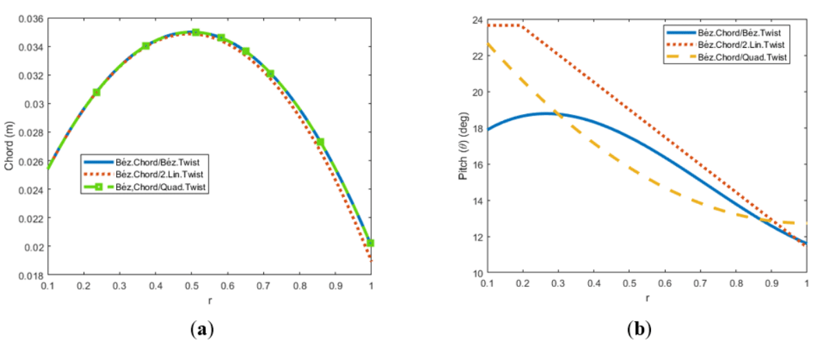
Figure 12 Combined optimizations of chord and twist for hovering
(a) Optimal chord distributions. (b) Optimal twist distributions.

Forward flight optimization

Chord optimization, constant pitch of 10 deg

Linear case and quadratic chord, 2 parameters: As it happened for hovering, the straight blade was the optimal solution for all the cases and velocities. Table 9 shows the parameters of the baseline rotor, the geometry achieved. For the quadratic case, the parameter ( a 2 ) MathType@MTEF@5@5@+= feaagKart1ev2aqatCvAUfeBSjuyZL2yd9gzLbvyNv2CaerbuLwBLn hiov2DGi1BTfMBaeXatLxBI9gBaerbd9wDYLwzYbItLDharqqtubsr 4rNCHbGeaGqk0dg9crFfpeea0xh9v8qiW7rqqrFfpeea0xe9Lq=Jc9 vqaqpepm0xbba9pwe9Q8fs0=yqaqpepae9pg0FirpepeKkFr0xfr=x fr=xb9adbaqaaeGaciGaaiaabeqaamaabaabaaGcbaaeaaaaaaaaa8 qadaqadaWdaeaapeGaamyya8aadaWgaaWcbaWdbiaaikdaa8aabeaa aOWdbiaawIcacaGLPaaaaaa@3BF0@ was zero for all analyzed cases. Hence, straight blade geometry is preferred rather than a quadratic tapered ( c root > c tip ) MathType@MTEF@5@5@+= feaagKart1ev2aqatCvAUfeBSjuyZL2yd9gzLbvyNv2CaerbuLwBLn hiov2DGi1BTfMBaeXatLxBI9gBaerbd9wDYLwzYbItLDharqqtubsr 4rNCHbGeaGqk0dg9crFfpeea0xh9v8qiW7rqqrFfpeea0xe9Lq=Jc9 vqaqpepm0xbba9pwe9Q8fs0=yqaqpepae9pg0FirpepeKkFr0xfr=x fr=xb9adbaqaaeGaciGaaiaabeqaamaabaabaaGcbaaeaaaaaaaaa8 qadaqadaWdaeaapeGaam4ya8aadaWgaaWcbaWdbiaadkhacaWGVbGa am4Baiaadshaa8aabeaak8qacqGH+aGpcaWGJbWdamaaBaaaleaape GaamiDaiaadMgacaWGWbaapaqabaaak8qacaGLOaGaayzkaaaaaa@444E@ distribution.

Vf(m/s)

Croot(m)

tap

P(W)

10

0.02

1

45.0791

15

0.02

1

83.1649

20 (*µx=0.0927)

0.02

1

202.2638

Table 9 1 linear segment chord distributions, parameters, and power requirements estimations for forward flight regime at three different speeds
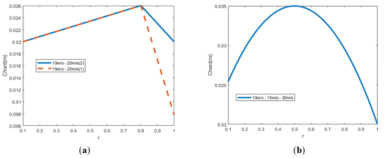
2 linear segments case, 4 parameters:

First differences appear. Table 10 gathers the results for hexagonal blades. Regarding to the case of 20 m/s, with the fixed constant pitch and the radius of the blade defined, no platforms could be found that provided the required thrust without violating the condition of ( μ x 0.1 ) MathType@MTEF@5@5@+= feaagKart1ev2aqatCvAUfeBSjuyZL2yd9gzLbvyNv2CaerbuLwBLn hiov2DGi1BTfMBaeXatLxBI9gBaerbd9wDYLwzYbItLDharqqtubsr 4rNCHbGeaGqk0dg9crFfpeea0xh9v8qiW7rqqrFfpeea0xe9Lq=Jc9 vqaqpepm0xbba9pwe9Q8fs0=yqaqpepae9pg0FirpepeKkFr0xfr=x fr=xb9adbaqaaeGaciGaaiaabeqaamaabaabaaGcbaaeaaaaaaaaa8 qadaqadaWdaeaapeGaeqiVd02damaaBaaaleaapeGaamiEaaWdaeqa aOWdbiabgwMiZkaaicdacaGGUaGaaGymaaGaayjkaiaawMcaaaaa@40EE@ . Figure 13(a) shows the distributions.

Vf(m/s)

Croot(m)

tap1

tap2

rperc

P(W)

ΔP( % ) MathType@MTEF@5@5@+= feaagKart1ev2aaatCvAUfeBSjuyZL2yd9gzLbvyNv2CaerbuLwBLn hiov2DGi1BTfMBaeXatLxBI9gBaerbd9wDYLwzYbItLDharqqtubsr 4rNCHbGeaGqk0dg9crFfpeea0xh9v8qiW7rqqrFfpeea0xe9Lq=Jc9 vqaqpepm0xbba9pwe9Q8fs0=yqaqpepae9pg0FirpepeKkFr0xfr=x fr=xb9adbaqaaeGaciGaaiaabeqaamaabaabaaGcbaqcLbsaqaaaaa aaaaWdbiaabs5acaqGqbGcpaWaaeWaaeaajugib8qacaqGLaaak8aa caGLOaGaayzkaaaaaa@3DAF@

10

0.02

1.3

1/1.3

0.8

42.5221

-5.67

15

0.02

1.3

0.3

0.8

76.9866

-7.43

(1) 20 (*µx=0.0924)

0.02

1.3

0.3

0.8

184.1586

-8.95

(2) 20(*µx=0.0959)

0.02

1.3

1/1.3

0.8

192.5949

-4.78

Table 10 2 linear segment chord distributions, parameters, and power requirements estimations for forward flight regime at three different speeds
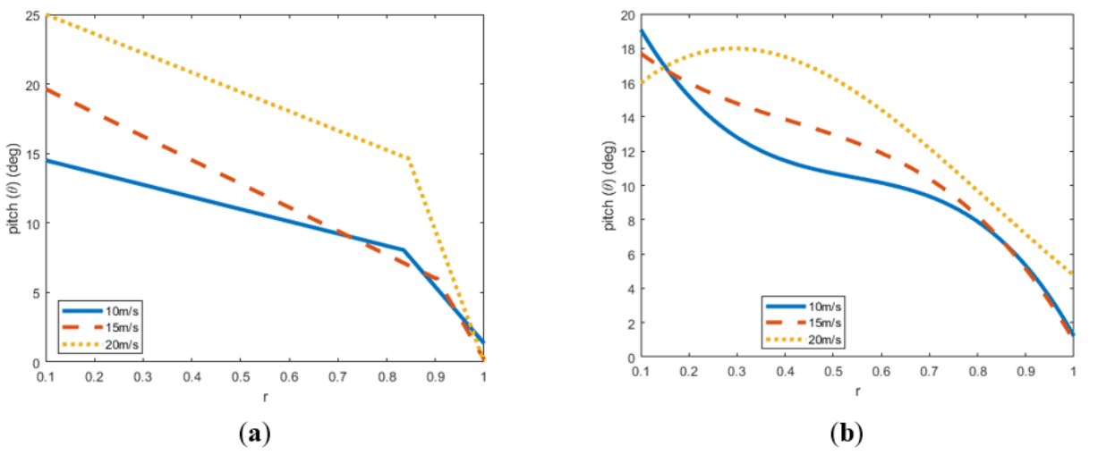
Figure 13 Isolated chord optimization for forward flight
(a) Optimal 2. linear chord distributions. (b) Optimal Bézier distributions.

Bézier cubic curve, 6 parameters:

The difference between the solutions is only the radial coordinate of the control points of the curve, however, the sensitivity of the function is not that big (Table 11), so the coordinates do not have an impact. Similarly to the previous case, the platform surface is increased, Figure 13(b).

Twist optimization, constant chord of 0.02 m

Vf(m/s)

Croot(m)

tap

r3

y4

r5

y6

P(W)

ΔP( % ) MathType@MTEF@5@5@+= feaagKart1ev2aaatCvAUfeBSjuyZL2yd9gzLbvyNv2CaerbuLwBLn hiov2DGi1BTfMBaeXatLxBI9gBaerbd9wDYLwzYbItLDharqqtubsr 4rNCHbGeaGqk0dg9crFfpeea0xh9v8qiW7rqqrFfpeea0xe9Lq=Jc9 vqaqpepm0xbba9pwe9Q8fs0=yqaqpepae9pg0FirpepeKkFr0xfr=x fr=xb9adbaqaaeGaciGaaiaabeqaamaabaabaaGcbaqcLbsaqaaaaa aaaaWdbiaabs5acaqGqbGcpaWaaeWaaeaajugib8qacaqGLaaak8aa caGLOaGaayzkaaaaaa@3DAF@

10

0.02

1

0.3802

0.04

0.7783

0.04

39.9319

-11.42

15

0.02

1

0.3831

0.04

0.7783

0.04

72.9050

-12.33

20 (*µx=0.097)

0.02

1

0.3177

0.0400

0.6076

0.04

187.374

-7.36

Table 11 Bézier cubic chord distributions, parameters, and power requirements estimations for forward flight regime at three different speeds
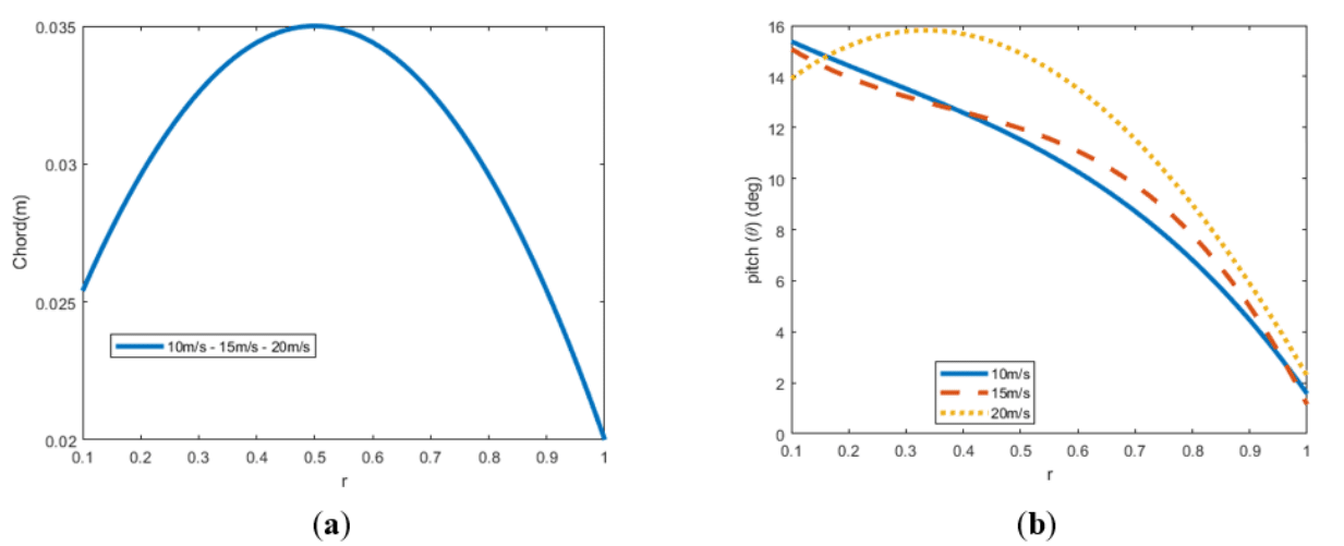
By contrast to the chord optimization, for which the optimal solution was barely the same regardless of the speed case. For twist, differences are found in the pitch variation between root and tip and, for some cases, in the curvature of the whole distribution.

Linear case, 2 parameters:

As it is frequent, the twist rate is negative. Moreover, for the case of 20 m/s, the differential pitch is smaller. More constant pitch is required due to high thrust demands. Regarding the other cases, pitch near the tip is barely zero, it is observed the influence of the tip losses. Those sections of the blade barely provide lift so a big pitch would only mean more drag without benefits for lift generation, Table 12, and Figure 14(a).

Quadratic case, 2 parameters:

Vf(m/s)

θroot(rad)

slp

P(W)

ΔP( % ) MathType@MTEF@5@5@+= feaagKart1ev2aaatCvAUfeBSjuyZL2yd9gzLbvyNv2CaerbuLwBLn hiov2DGi1BTfMBaeXatLxBI9gBaerbd9wDYLwzYbItLDharqqtubsr 4rNCHbGeaGqk0dg9crFfpeea0xh9v8qiW7rqqrFfpeea0xe9Lq=Jc9 vqaqpepm0xbba9pwe9Q8fs0=yqaqpepae9pg0FirpepeKkFr0xfr=x fr=xb9adbaqaaeGaciGaaiaabeqaamaabaabaaGcbaqcLbsaqaaaaa aaaaWdbiaabs5acaqGqbGcpaWaaeWaaeaajugib8qacaqGLaaak8aa caGLOaGaayzkaaaaaa@3DAF@

10

0.3145

-0.2896

39.8667

-11.56

15

0.3717

-0.3555

65.7039

-20.99

20

0.2948

-0.1649

172.4304

-14.75

Table 12 1 linear segment twist distributions, parameters, and power requirements estimations for forward flight regime at three different speeds

Figure 14 Isolated twist optimization for forward flight
(a) Optimal 2 linear twist distributions. (b) Optimal Bézier distributions.

Like in the linear case, increasing the forward speed tends to result in a flatter pitch distribution. See Table 13 and Figure 14(b).

Vf(m/s)

θroot(rad)

slp1

slp2

rperc

P(W)

ΔP( % ) MathType@MTEF@5@5@+= feaagKart1ev2aaatCvAUfeBSjuyZL2yd9gzLbvyNv2CaerbuLwBLn hiov2DGi1BTfMBaeXatLxBI9gBaerbd9wDYLwzYbItLDharqqtubsr 4rNCHbGeaGqk0dg9crFfpeea0xh9v8qiW7rqqrFfpeea0xe9Lq=Jc9 vqaqpepm0xbba9pwe9Q8fs0=yqaqpepae9pg0FirpepeKkFr0xfr=x fr=xb9adbaqaaeGaciGaaiaabeqaamaabaabaaGcbaqcLbsaqaaaaa aaaaWdbiaabs5acaqGqbGcpaWaaeWaaeaajugib8qacaqGLaaak8aa caGLOaGaayzkaaaaaa@3DAF@

10

0.2532

-0.1120

-0.1178

0.8323

38.9792

-13.53

15

0.3426

-0.2374

-0.1021

0.8997

64.2680

-22.72

20

0.4363

-0.18

-0.2563

0.8420

150.5187

-25.6

Table 13 Quadratic twist, parameters, and power requirements estimations for forward flight regime at three different speeds

2 linear cases, 4 parameters:

All solutions share the same behavior. First segment’s slope is less negative than near the tip. Near the tip, a steep pitch reduction is observed for all the cases until almost zero pitch, therefore, reducing the lift in the tip. Results are showed in Table 14 and Figure 15(a).

Vf(m/s)

θroot(rad)

slp1

slp2

rperc

P(W)

ΔP( % ) MathType@MTEF@5@5@+= feaagKart1ev2aaatCvAUfeBSjuyZL2yd9gzLbvyNv2CaerbuLwBLn hiov2DGi1BTfMBaeXatLxBI9gBaerbd9wDYLwzYbItLDharqqtubsr 4rNCHbGeaGqk0dg9crFfpeea0xh9v8qiW7rqqrFfpeea0xe9Lq=Jc9 vqaqpepm0xbba9pwe9Q8fs0=yqaqpepae9pg0FirpepeKkFr0xfr=x fr=xb9adbaqaaeGaciGaaiaabeqaamaabaabaaGcbaqcLbsaqaaaaa aaaaWdbiaabs5acaqGqbGcpaWaaeWaaeaajugib8qacaqGLaaak8aa caGLOaGaayzkaaaaaa@3DAF@

10

0.2532

-0.1120

-0.1178

0.8323

38.9792

-13.53

15

0.3426

-0.2374

-0.1021

0.8997

64.2680

-22.72

20

0.4363

-0.18

-0.2563

0.8420

150.5187

-25.6

Table 14 2 linear segment twist distributions, parameters, and power requirements estimations for forward flight regime at three different speeds

Figure 15 Combined optimizations of Bezier chord and Bezier twist distributions for forward flight
(a) Optimal chord distributions (b) Optimal twist distributions.

Bézier cubic curve, 6 parameters:

For the two first speeds analyzed show similar results to the previous ones, a clear negative twist, the middle zone of the blade shows flatter distributions whereas near to the tip the pitch approaches to zero rapidly. By contrast, the case of 20 m/s shows a particular opposite tendency for sections closer to the root where the pitch is increased. See the results in Table 15 and Figure 15(b).

Vf(m/s)

θroot

θtip

r3

y4

r5

y6

P(W)

ΔP( % ) MathType@MTEF@5@5@+= feaagKart1ev2aaatCvAUfeBSjuyZL2yd9gzLbvyNv2CaerbuLwBLn hiov2DGi1BTfMBaeXatLxBI9gBaerbd9wDYLwzYbItLDharqqtubsr 4rNCHbGeaGqk0dg9crFfpeea0xh9v8qiW7rqqrFfpeea0xe9Lq=Jc9 vqaqpepm0xbba9pwe9Q8fs0=yqaqpepae9pg0FirpepeKkFr0xfr=x fr=xb9adbaqaaeGaciGaaiaabeqaamaabaabaaGcbaqcLbsaqaaaaa aaaaWdbiaabs5acaqGqbGcpaWaaeWaaeaajugib8qacaqGLaaak8aa caGLOaGaayzkaaaaaa@3DAF@

10

0.4342

0.0213

0.2317

0.0336

0.7783

0.3128

39.0150

-13.45

15

0.3517

0.0165

0.2467

0.1827

0.6724

0.2980

64.2927

-22.69

20

0.2290

0.0831

0.2428

0.4363

0.5582

0.2157

145.4929

-28.06

Table 15 Bézier cubic twist distributions, parameters, and power estimations for forward flight regime at three different speeds

Twist and chord optimization

Bézier chord and Bézier twist, 12 parameters:

The chord distributions obtained are identical to those obtained through isolated resolution, in which the optimal distribution was increasing the platform area. Parameters and the representation are in Table 16 and Figure 16.

Vf(m/s)

Croot

tap

r3

y4

r5

y6

P(W)

ΔP( % ) MathType@MTEF@5@5@+= feaagKart1ev2aaatCvAUfeBSjuyZL2yd9gzLbvyNv2CaerbuLwBLn hiov2DGi1BTfMBaeXatLxBI9gBaerbd9wDYLwzYbItLDharqqtubsr 4rNCHbGeaGqk0dg9crFfpeea0xh9v8qiW7rqqrFfpeea0xe9Lq=Jc9 vqaqpepm0xbba9pwe9Q8fs0=yqaqpepae9pg0FirpepeKkFr0xfr=x fr=xb9adbaqaaeGaciGaaiaabeqaamaabaabaaGcbaqcLbsaqaaaaa aaaaWdbiaabs5acaqGqbGcpaWaaeWaaeaajugib8qacaqGLaaak8aa caGLOaGaayzkaaaaaa@3DAF@

10

0.02

1

0.26

0.04

0.6543

0.04

33.4445

-25.8

15

0.02

1

0.26

0.0400

0.6543

0.04

53.7427

-35.4

20

0.02

1

0.4259

0.0400

0.7727

0.04

131.51

-34.98

Table 16 Combined twist and chord optimization, chord distribution parameters, and power requirements estimations for forward flight regime at three different speeds, optimization case 1

Figure 16 Combined optimizations of Bezier chord and quadratic twist distributions for forward flight
(a) Optimal chord distributions (b) Optimal twist distributions.

Optimal twist distributions show slight differences compared to those obtained without chord optimization, Table 17. Two first distributions are quite similar one to the other. Apart from that, the pitch for 20 m/s case, decreases faster near to the tip than it was for the previous study. Distributions are displayed in Figure 16.

Vf(m/s)

θroot

θtip

r7

y8

r9

y10

P(W)

ΔP( % ) MathType@MTEF@5@5@+= feaagKart1ev2aaatCvAUfeBSjuyZL2yd9gzLbvyNv2CaerbuLwBLn hiov2DGi1BTfMBaeXatLxBI9gBaerbd9wDYLwzYbItLDharqqtubsr 4rNCHbGeaGqk0dg9crFfpeea0xh9v8qiW7rqqrFfpeea0xe9Lq=Jc9 vqaqpepm0xbba9pwe9Q8fs0=yqaqpepae9pg0FirpepeKkFr0xfr=x fr=xb9adbaqaaeGaciGaaiaabeqaamaabaabaaGcbaqcLbsaqaaaaa aaaaWdbiaabs5acaqGqbGcpaWaaeWaaeaajugib8qacaqGLaaak8aa caGLOaGaayzkaaaaaa@3DAF@

10

0.2871

0.0273

0.3850

0.2192

0.6543

0.2122

33.4445

-25.8

15

0.2921

0.02

0.3850

0.1758

0.6543

0.277

53.7427

-35.4

20

0.2074

0.0396

0.4259

0.3474

0.7727

0.2641

131.51

-34.98

Table 17 Combined twist and chord optimization, twist distribution parameters, and power estimations for forward flight regime at three different speeds, optimization case 1

Quadratic twist and Bezier chord, 8 parameters:

Only the 3rd considered speed scenario shows interesting variations. For detailed results check Tables 18 & 19 and Figure 17.

Vf(m/s)

Croot

tap

r3

y4

r5

y6

P(W)

ΔP( % ) MathType@MTEF@5@5@+= feaagKart1ev2aaatCvAUfeBSjuyZL2yd9gzLbvyNv2CaerbuLwBLn hiov2DGi1BTfMBaeXatLxBI9gBaerbd9wDYLwzYbItLDharqqtubsr 4rNCHbGeaGqk0dg9crFfpeea0xh9v8qiW7rqqrFfpeea0xe9Lq=Jc9 vqaqpepm0xbba9pwe9Q8fs0=yqaqpepae9pg0FirpepeKkFr0xfr=x fr=xb9adbaqaaeGaciGaaiaabeqaamaabaabaaGcbaqcLbsaqaaaaa aaaaWdbiaabs5acaqGqbGcpaWaaeWaaeaajugib8qacaqGLaaak8aa caGLOaGaayzkaaaaaa@3DAF@

10

0.02

1

0.2317

0.0400

0.7783

0.04

35.2283

-21.85

15

0.02

1

0.2528

0.0400

0.6054

0.04

59.9568

-27.9

20

0.01

0.2002

0.3177

0.0400

0.6076

0.04

176.98

-12.5

Table 18 Combined twist and chord optimization, chord distribution parameters, and power requirements estimations for forward flight regime at three different speeds, optimization case 2
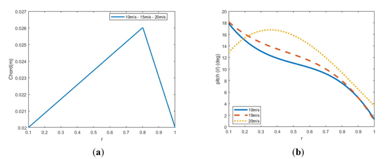
Vf(m/s)

θroot

a1

P(W)

ΔP( % ) MathType@MTEF@5@5@+= feaagKart1ev2aaatCvAUfeBSjuyZL2yd9gzLbvyNv2CaerbuLwBLn hiov2DGi1BTfMBaeXatLxBI9gBaerbd9wDYLwzYbItLDharqqtubsr 4rNCHbGeaGqk0dg9crFfpeea0xh9v8qiW7rqqrFfpeea0xe9Lq=Jc9 vqaqpepm0xbba9pwe9Q8fs0=yqaqpepae9pg0FirpepeKkFr0xfr=x fr=xb9adbaqaaeGaciGaaiaabeqaamaabaabaaGcbaqcLbsaqaaaaa aaaaWdbiaabs5acaqGqbGcpaWaaeWaaeaajugib8qacaqGLaaak8aa caGLOaGaayzkaaaaaa@3DAF@

10

0.4363

0.3511

35.2833

-21.85

15

0.4361

0.3316

59.9568

-27.9

20

0.2667

0.0745

176.98

-12.5

Table 19 Combined twist and chord optimization, twist distribution parameters, and power requirements estimations for forward flight regime at three different speeds, optimization case 2

Figure 17 Combined optimizations of 2 linear chord and Bezier twist distributions for forward flight
(a) Optimal chord distributions (b) Optimal twist distributions.

In terms of pitch. Again, 20 m/s case is the one showing relevant discrepancies to previous results. Before, for the quadratic distribution it was already noticed that the distribution was flatter for this speed, however, now with the addition of the chord distribution, the parabola it is even flatter, and the pitch remains on average quite constant over the blade. Also, this can be related with the necessity if a smaller blade surface for generating the required thrust, mainly because on average the pitch is bigger, so more lift is produced.

Bézier twist and 2 linear chord, 10 parameters:

As it happened during the optimization of chords following this distribution, the tendencies are again to increase the surface available for lift generation creating hexagonal blades. Results in Table 20 & 21 and Figure 18.

Vf(m/s)

Croot

tap1

tap2

rperc

P(W)

ΔP( % ) MathType@MTEF@5@5@+= feaagKart1ev2aaatCvAUfeBSjuyZL2yd9gzLbvyNv2CaerbuLwBLn hiov2DGi1BTfMBaeXatLxBI9gBaerbd9wDYLwzYbItLDharqqtubsr 4rNCHbGeaGqk0dg9crFfpeea0xh9v8qiW7rqqrFfpeea0xe9Lq=Jc9 vqaqpepm0xbba9pwe9Q8fs0=yqaqpepae9pg0FirpepeKkFr0xfr=x fr=xb9adbaqaaeGaciGaaiaabeqaamaabaabaaGcbaqcLbsaqaaaaa aaaaWdbiaabs5acaqGqbGcpaWaaeWaaeaajugib8qacaqGLaaak8aa caGLOaGaayzkaaaaaa@3DAF@

10

0.02

1.3

1/1.3

0.8

36.4908

-19.05

15

0.02

1.3

1/1.3

0.8

59.7391

-28.17

20

0.02

1.3

1/1.3

0.8

132.6546

-34.41

Table 20 Combined twist and chord optimization, chord distribution parameters, and power requirements estimations for forward flight regime at three different speeds, optimization case 3

Vf(m/s)

θroot

θtip

r3

y4

r5

y6

P(W)

ΔP( % ) MathType@MTEF@5@5@+= feaagKart1ev2aaatCvAUfeBSjuyZL2yd9gzLbvyNv2CaerbuLwBLn hiov2DGi1BTfMBaeXatLxBI9gBaerbd9wDYLwzYbItLDharqqtubsr 4rNCHbGeaGqk0dg9crFfpeea0xh9v8qiW7rqqrFfpeea0xe9Lq=Jc9 vqaqpepm0xbba9pwe9Q8fs0=yqaqpepae9pg0FirpepeKkFr0xfr=x fr=xb9adbaqaaeGaciGaaiaabeqaamaabaabaaGcbaqcLbsaqaaaaa aaaaWdbiaabs5acaqGqbGcpaWaaeWaaeaajugib8qacaqGLaaak8aa caGLOaGaayzkaaaaaa@3DAF@

10

0.3861

0.0221

0.4493

0.0951

0.7398

0.2817

36.4908

-19.05

15

0.3694

0.0180

0.3268

0.1647

0.7384

0.2883

59.7391

-28.17

20

0.1535

0.0635

0.4403

0.4363

0.6679

0.2279

132.6546

-34.41

Table 21 Combined twist and chord optimization, twist distribution parameters, and power requirements estimations for forward flight regime at three different speeds, optimization case 3

Figure 18 Fluid domains and boundary conditions
(a) Hovering simulations (b) Forward flight simulations.

For the pitch, the distributions remain quite the same to the previous ones.

In terms of power reduction, all cases show enhanced performance compared to the baseline. Moreover, the combination of chord and twist seems to be better than just modifying one parameter, as it happens with large scale rotors. However, obtained results show large improvements in terms of power consumption. Those results might be quite optimistic, and they must be verified against CFD simulations.

CFD simulations

Set up and previous studies

As previously mentioned, CFD simulations are used for verification of the obtained results and models. Complex 3D phenomena and other aspects difficult to quantifies theoretically can be approached with these tools. Within the domain of CFD, there are usually more than one approach for the same kind of problem. As stated during the introduction, rotary flows can be treated with three methods. The setup of the simulations as well as the fluid domain geometry depend on the course of action for tackling up the issue. Among the possible alternatives, Multiple reference frame (MRF) has been chosen for solving hover simulations, as it was done by R.Cagnato.1 This strategy allows simulating the problem in quasi-steady approach without needing transient simulations by using a static absolute frame and a rotational frame. MRF can only be applied to constant rotational flows and Navier-Stokes equations are solved considering the relative velocities between frames.1

On the other hand, for addressing forward flight, transient simulations are required. Sliding mesh will be used. Prior to this, other researchers obtained satisfactory results by this method.7 Sliding mesh is selected since forward flight flow requires a more accurate time solution due to flow variation over the revolution. Concerning to the turbulent model, based on the preferences in prior projects, k − ω SST has been chosen for hovering and forward flight. This model can transition automatically from viscous sublayer to logarithmic layer. Furthermore, it is suitable for low Reynolds regime, and it is possible to activate a third equation for addressing the possible transition between laminar to turbulent flow.22

Fluid domain configuration

For hover simulations, two cylindrical domains are created: one surrounds the rotor and represents the fluid zone linked to the rotary reference frame, while the other represents the static zone and is linked to the absolute frame of reference. The dimensions, Table 22, of both zones are defined based on the dimensional analysis available in.17

Domain Zone

upper length (m)

bottom length(m)

Radius(m)

Outer Cylinder

2.5

4.5

4

Inner Cylinder

0.3

0.3

0.35

Table 22 CFD hovering simulations fluid domain final dimensions

For forward flight simulations. The rotary domain is represented by a cylinder. However, the static domain is a rectangular prism. Moreover, an extra rectangular box was used for grid refinement tasks near the interface between domains. The dimensions have been determined based on prior studies.7,23 Table 23 shows the dimensions of the domains.

Domain Zone

Height(m)

thickness/radius(m)

Length(m)

Outer box

8

4

12

Refinement box

2

1.5

4

Inner Cylinder

0.066

0.44

-

Table 23 CFD hovering simulations fluid domain final dimensions

Boundary conditions and set up

The top base of the static cylinder is designated as a pressure inlet, while the bottom is set as a pressure outlet. Symmetry conditions are applied to the lateral surface to prevent perpendicular flow or convection. The shared surface between fluid zones is declared as an interface and rotor surface as a moving wall with no-slip condition and zero relative speed to adjacent cell zones. The rest of set up configurations follows R. Cagnato procedure,1 which are based on Ansys guidelines. Computations are performed using absolute reference frame with Pressure solver, velocity-pressure coupling is solved using the COUPLED method because of its robustness converging. Discretization is set using second order upwind for more accuracy, except for pressure, which uses the PRESTO scheme.

For forward flight simulations, all faces except the backward are set as velocity inlets, defined by the flow magnitude and direction, allowing consideration of various rotor inclinations. The backward surface is a pressure outlet. Inner box solid is just used for grid discretization. Static-rotational cylinder iteration is defined as an interface and rotor surface is set as a moving wall with no-slip condition and zero relative velocity to adjacent cell zone. COUPLED is again selected to solve the differential equation system, with second order upwind used for discretization. Figure 19 shows the defined fluid domains and the boundary conditions.
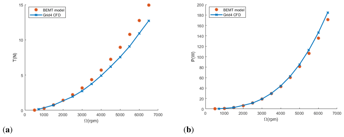
Figure 19 Comparison between model estimations and CFD simulations of the baseline rotor at hovering flight (a) Thrust (N) versus rotational speed ( Ω( rpm ) ) MathType@MTEF@5@5@+= feaagKart1ev2aqatCvAUfeBSjuyZL2yd9gzLbvyNv2CaerbuLwBLn hiov2DGi1BTfMBaeXatLxBI9gBaerbd9wDYLwzYbItLDharqqtubsr 4rNCHbGeaGqk0dg9crFfpeea0xh9v8qiW7rqqrFfpeea0xe9Lq=Jc9 vqaqpepm0xbba9pwe9Q8fs0=yqaqpepae9pg0FirpepeKkFr0xfr=x fr=xb9adbaqaaeGaciGaaiaabeqaamaabaabaaGcbaWaaeWaaeaaju gibabaaaaaaaaapeGaaeyQdOWdamaabmaabaqcLbsapeGaaeOCaiaa bchacaqGTbaak8aacaGLOaGaayzkaaaacaGLOaGaayzkaaaaaa@40AB@ . (b) Power (W) versus rotational speed ( Ω( rpm ) ) MathType@MTEF@5@5@+= feaagKart1ev2aqatCvAUfeBSjuyZL2yd9gzLbvyNv2CaerbuLwBLn hiov2DGi1BTfMBaeXatLxBI9gBaerbd9wDYLwzYbItLDharqqtubsr 4rNCHbGeaGqk0dg9crFfpeea0xh9v8qiW7rqqrFfpeea0xe9Lq=Jc9 vqaqpepm0xbba9pwe9Q8fs0=yqaqpepae9pg0FirpepeKkFr0xfr=x fr=xb9adbaqaaeGaciGaaiaabeqaamaabaabaaGcbaWaaeWaaeaaju gibabaaaaaaaaapeGaaeyQdOWdamaabmaabaqcLbsapeGaaeOCaiaa bchacaqGTbaak8aacaGLOaGaayzkaaaacaGLOaGaayzkaaaaaa@40AB@ .

Grids and time step analysis

For both cases, an unstructured grid was chosen due to its semi-automatic generation and proven ability to yield good results. To ensure proper capture of the boundary layer, inflation with multiple prismatic layers was applied around the rotor blades. The first layer thickness was set to 5e-6 meters to maintain a wall y+ ∼ 1.

Grid analysis was performed for both simulations to ensure grid independence and reach a balance between time and accuracy, crucial for forward flight simulations, which demanded a high computational cost. Results are shown in Table 24 &25.

Grid

N.Elements(×106)

T (N)

ΔT(%)

Torque (Nm)

ΔTorque(%)

Coarse

1.4

8.78

3.25

0.27

16.12

Medium

3.5

9

0.826

0.242

4.086

Medium-Fine

5

9.05

0.276

0.235

1.07

Fine

6

9.075

-

0.2325

-

Table 24 CFD hovering simulations grid analysis at 5000 rpm

Step

T (N)

ΔT(%)

Trq (Nm)

ΔTorque(%)

 = 2

5.302

0.263

0.07764

0.414

 = 1

5.292

0.415

0.07727

0.647

 = 0.7

5.316

-

0.07732

-

Table 25 CFD forward flight simulations step time analysis

It is concluded that a medium-fine grid should be sufficient, as the variations with the finest mesh are lower than 5% for both cases.

Moving on to forward flight grids, it must be checked the grid independence and the required time step. These simulations must be done transiently, which requires high simulation time. Additionally, to prevent convergence issues and ensure stability, it is mandatory to use an appropriate time step. Priorly, in,8 for hovering sliding mesh simulation, a time step equivalent to ψ=4 MathType@MTEF@5@5@+= feaagKart1ev2aaatCvAUfeBSjuyZL2yd9gzLbvyNv2CaerbuLwBLn hiov2DGi1BTfMBaeXatLxBI9gBaerbd9wDYLwzYbItLDharqqtubsr 4rNCHbGeaGqk0dg9crFfpeea0xh9v8qiW7rqqrFfpeea0xe9Lq=Jc9 vqaqpepm0xbba9pwe9Q8fs0=yqaqpepae9pg0FirpepeKkFr0xfr=x fr=xb9adbaqaaeGaciGaaiaabeqaamaabaabaaGcbaaeaaaaaaaaa8 qacqaHipqEcqGH9aqpcaaI0aaaaa@3BC3@ deg was enough. However, in forward flight, other researchers performed simulations with smaller time steps within the range of Δψ=1 MathType@MTEF@5@5@+= feaagKart1ev2aaatCvAUfeBSjuyZL2yd9gzLbvyNv2CaerbuLwBLn hiov2DGi1BTfMBaeXatLxBI9gBaerbd9wDYLwzYbItLDharqqtubsr 4rNCHbGeaGqk0dg9crFfpeea0xh9v8qiW7rqqrFfpeea0xe9Lq=Jc9 vqaqpepm0xbba9pwe9Q8fs0=yqaqpepae9pg0FirpepeKkFr0xfr=x fr=xb9adbaqaaeGaciGaaiaabeqaamaabaabaaGcbaaeaaaaaaaaa8 qacqqHuoarcqaHipqEcqGH9aqpcaaIXaaaaa@3D26@ deg.7 Results of the step-time analysis showed in Table 26.

Grid

N.Elements(×106)

T (N)

ΔT(%)

Torque (Nm)

ΔTorque(%)

Coarse

4

5.42

2.5

0.0779

1.04

Medium

6

5.29

0.038

0.07715

0.065

Fine

8.7

5.288

-

0.0771

-

Table 26 CFD forward flight simulations grid analysis

After the studies, it is concluded that a medium grid combined with a time step of Δψ=2 MathType@MTEF@5@5@+= feaagKart1ev2aaatCvAUfeBSjuyZL2yd9gzLbvyNv2CaerbuLwBLn hiov2DGi1BTfMBaeXatLxBI9gBaerbd9wDYLwzYbItLDharqqtubsr 4rNCHbGeaGqk0dg9crFfpeea0xh9v8qiW7rqqrFfpeea0xe9Lq=Jc9 vqaqpepm0xbba9pwe9Q8fs0=yqaqpepae9pg0FirpepeKkFr0xfr=x fr=xb9adbaqaaeGaciGaaiaabeqaamaabaabaaGcbaaeaaaaaaaaa8 qacqqHuoarcqaHipqEcqGH9aqpcaaIYaaaaa@3D27@ deg is a compromise solution. With this combination, the time required per simulation (four full rotations until report convergence) was approximately 19 h.

Discussion of results: Model and CFD comparison

Hover simulations

The baseline rotor was simulated at several rotational speeds. In general, model and CFD simulations show similar results. The model based on BEMT seems suitable for estimating rotor performance capacities in hover. The theoretical model overestimates thrust capacities and under predicts power requirements, still, good predictions are yielded. Figure 20 shows the results and the inflow distribution is analyzed in Figure 21.
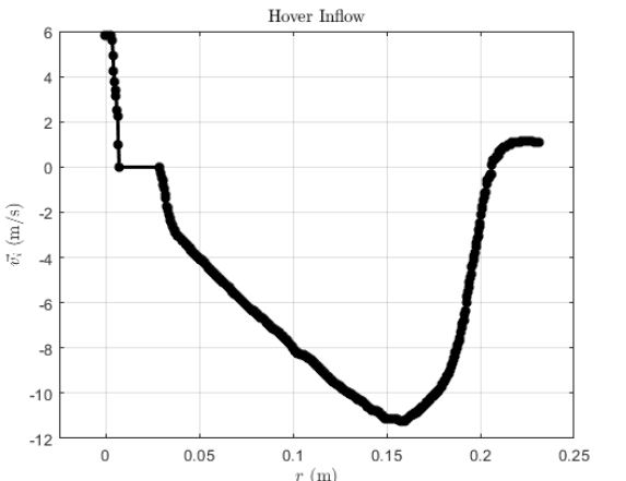
Figure 20 Inflow speed distribution ( v i ) MathType@MTEF@5@5@+= feaagKart1ev2aqatCvAUfeBSjuyZL2yd9gzLbvyNv2CaerbuLwBLn hiov2DGi1BTfMBaeXatLxBI9gBaerbd9wDYLwzYbItLDharqqtubsr 4rNCHbGeaGqk0dg9crFfpeea0xh9v8qiW7rqqrFfpeea0xe9Lq=Jc9 vqaqpepm0xbba9pwe9Q8fs0=yqaqpepae9pg0FirpepeKkFr0xfr=x fr=xb9adbaqaaeGaciGaaiaabeqaamaabaabaaGcbaWaaeWaaeaada WhcaqaaabaaaaaaaaapeGaamODa8aadaWgaaWcbaWdbiaadMgaa8aa beaaaOGaay51GaaacaGLOaGaayzkaaaaaa@3DBC@ along the blade from CFD simulations at hovering.
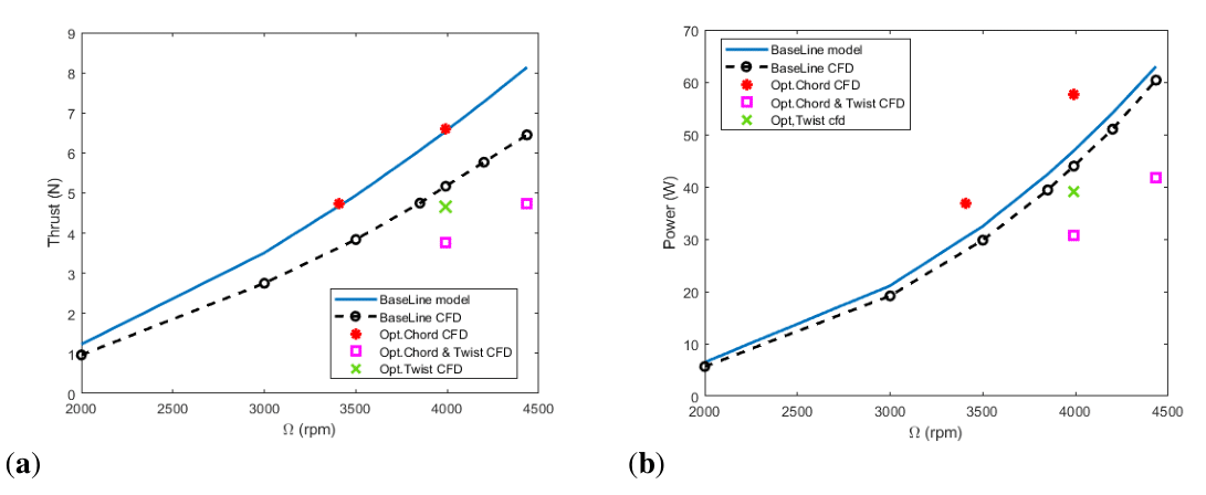
Figure 21 Comparison between model estimations and CFD simulations of the baseline rotor and some optimal rotors at forward flight
(a) Thrust (N) versus rotational speed ( Ω( rpm ) ) MathType@MTEF@5@5@+= feaagKart1ev2aqatCvAUfeBSjuyZL2yd9gzLbvyNv2CaerbuLwBLn hiov2DGi1BTfMBaeXatLxBI9gBaerbd9wDYLwzYbItLDharqqtubsr 4rNCHbGeaGqk0dg9crFfpeea0xh9v8qiW7rqqrFfpeea0xe9Lq=Jc9 vqaqpepm0xbba9pwe9Q8fs0=yqaqpepae9pg0FirpepeKkFr0xfr=x fr=xb9adbaqaaeGaciGaaiaabeqaamaabaabaaGcbaWaaeWaaeaaju gibabaaaaaaaaapeGaaeyQdOWdamaabmaabaqcLbsapeGaaeOCaiaa bchacaqGTbaak8aacaGLOaGaayzkaaaacaGLOaGaayzkaaaaaa@40AB@ (b) Power (W) versus rotational speed ( Ω( rpm ) ) MathType@MTEF@5@5@+= feaagKart1ev2aqatCvAUfeBSjuyZL2yd9gzLbvyNv2CaerbuLwBLn hiov2DGi1BTfMBaeXatLxBI9gBaerbd9wDYLwzYbItLDharqqtubsr 4rNCHbGeaGqk0dg9crFfpeea0xh9v8qiW7rqqrFfpeea0xe9Lq=Jc9 vqaqpepm0xbba9pwe9Q8fs0=yqaqpepae9pg0FirpepeKkFr0xfr=x fr=xb9adbaqaaeGaciGaaiaabeqaamaabaabaaGcbaWaaeWaaeaaju gibabaaaaaaaaapeGaaeyQdOWdamaabmaabaqcLbsapeGaaeOCaiaa bchacaqGTbaak8aacaGLOaGaayzkaaaacaGLOaGaayzkaaaaaa@40AB@ . /p>

The induced speed distribution shows the effect of the hub, near to the root the induced speed goes to zero. Moreover, it is observed the presence of tip vortexes, there is an upward inflow at the tips because of the circulating flow due to the difference of pressure between bottom and upper zones.

Forward flight simulations

The baseline rotor was simulated at multiple rotational speeds to obtain the evolution of thrust and power at different pilot inputs. Additionally, the best optimal geometries were simulated at the rotational speed estimated for providing enough thrust for the drone model and at the same operational speed than the baseline. It is observed that the model is overestimating the thrust with errors of the order of 20%, Figure 22.
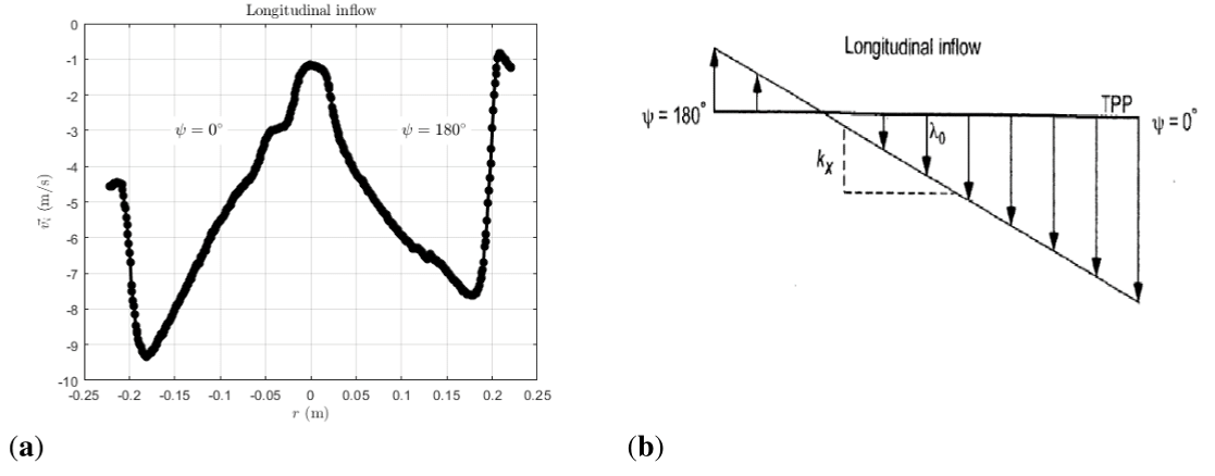
Figure 22 Comparison between inflows distributions from CFD simulations and theoretical lineal model16 at forward flight
(a) CFD longitudinal inflow ( v i ( m/s ) ) MathType@MTEF@5@5@+= feaagKart1ev2aqatCvAUfeBSjuyZL2yd9gzLbvyNv2CaerbuLwBLn hiov2DGi1BTfMBaeXatLxBI9gBaerbd9wDYLwzYbItLDharqqtubsr 4rNCHbGeaGqk0dg9crFfpeea0xh9v8qiW7rqqrFfpeea0xe9Lq=Jc9 vqaqpepm0xbba9pwe9Q8fs0=yqaqpepae9pg0FirpepeKkFr0xfr=x fr=xb9adbaqaaeGaciGaaiaabeqaamaabaabaaGcbaWaaeWaaeaada WhcaqaaabaaaaaaaaapeGaamODa8aadaWgaaWcbaWdbiaadMgaa8aa beaaaOGaay51GaWaaeWaaeaapeGaamyBaiaac+cacaWGZbaapaGaay jkaiaawMcaaaGaayjkaiaawMcaaaaa@4201@ . (b) Theoretical longitudinal linear inflow distribution.

Overestimation of thrust may be related to some sources of error. Firstly, as it was pointed out, XFOIL estimations for airfoil aerodynamic coefficients tends to be optimistic with lift capabilities and stall point prediction, as it can be observed in Figure 1. Besides that, the model and the simulations tend to diverge as rotational speed is increased, already during optimization problems with the applicability of the theory were observed, since the theory can only be applied for µx0.1 MathType@MTEF@5@5@+= feaagKart1ev2aaatCvAUfeBSjuyZL2yd9gzLbvyNv2CaerbuLwBLn hiov2DGi1BTfMBaeXatLxBI9gBaerbd9wDYLwzYbItLDharqqtubsr 4rNCHbGeaGqk0dg9crFfpeea0xh9v8qiW7rqqrFfpeea0xe9Lq=Jc9 vqaqpepm0xbba9pwe9Q8fs0=yqaqpepae9pg0FirpepeKkFr0xfr=x fr=xb9adbaqaaeGaciGaaiaabeqaamaabaabaaGcbaaeaaaaaaaaa8 qacaWG1cGaamiEaiabgwMiZkaaicdacaGGUaGaaGymaaaa@3E55@ . The operational speeds computed for each of the optimized rotors are closed to this limit of 0.1. Finally, the model is being applied for high pitch of the rotor, whereas when the theory is applied to large scale rotors for which the rotor pitch is usually a small angle. The bigger the inclination, the closer to an axial flight regime. Moreover, it is observed that the over-prediction of thrust is even bigger for the rotor geometries with variable pitch along the blades. As seen in the analysis of the optimized rotors, the twist distributions lead to very low pitch angles near to the tip due to the presence of losses, however, this is affecting considerably to the lift generation and simulations are not reflecting the estimated reduction in power by decreasing the pitch.

If the power requirements are compared, Table 27, it is observed that some of the geometries, that were supposed to enhance the baseline capabilities, are far for reaching the predicted improvements, particularly for the cases related with twist optimization.


Base Line

Béz.Chord

Bez. Chord/Twist

2 Lin.Twist

Power (W)

39.4

37.08

39.08

41.62

ΔP(%)

-

-5.88

-0.8

+5.6

Table 27 Power requirements comparison for the studied rotors

The optimization of the chord distribution provides a benefit in terms of power requirements. However, the rotor with variable pitch and constant chord does not improve the baseline and the combination of chord and twist shows negligible improvements. The improvement predictions of the model were only achieved for the chord optimization.

During the simulations, it was obtained the induced speed over the blades at multiple azimuth positions. As explained, the inflow was assumed to be linear. However, at the simulations, high non-uniform inflows were obtained. The inflow is far from the linear distribution assumed for longitudinal ( ψ=0,180 deg ) MathType@MTEF@5@5@+= feaagKart1ev2aaatCvAUfeBSjuyZL2yd9gzLbvyNv2CaerbuLwBLn hiov2DGi1BTfMBaeXatLxBI9gBaerbd9wDYLwzYbItLDharqqtubsr 4rNCHbGeaGqk0dg9crFfpeea0xh9v8qiW7rqqrFfpeea0xe9Lq=Jc9 vqaqpepm0xbba9pwe9Q8fs0=yqaqpepae9pg0FirpepeKkFr0xfr=x fr=xb9adbaqaaeGaciGaaiaabeqaamaabaabaaGcbaWaaeWaaeaaqa aaaaaaaaWdbiabeI8a5jabg2da9iaaicdacaGGSaGaaGymaiaaiIda caaIWaGaaeiiaiaadsgacaWGLbGaam4zaaWdaiaawIcacaGLPaaaaa a@43A0@ and lateral (90,270 deg) positions, as depicted in Figures 23 &24.
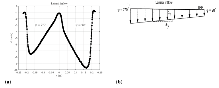
Figure 23 Comparison between inflows distributions from CFD simulations and theoretical lineal model16 at forward flight:
(a) CFD lateral inflow ( v i ( m/s ) ) MathType@MTEF@5@5@+= feaagKart1ev2aqatCvAUfeBSjuyZL2yd9gzLbvyNv2CaerbuLwBLn hiov2DGi1BTfMBaeXatLxBI9gBaerbd9wDYLwzYbItLDharqqtubsr 4rNCHbGeaGqk0dg9crFfpeea0xh9v8qiW7rqqrFfpeea0xe9Lq=Jc9 vqaqpepm0xbba9pwe9Q8fs0=yqaqpepae9pg0FirpepeKkFr0xfr=x fr=xb9adbaqaaeGaciGaaiaabeqaamaabaabaaGcbaWaaeWaaeaada WhcaqaaabaaaaaaaaapeGaamODa8aadaWgaaWcbaWdbiaadMgaa8aa beaaaOGaay51GaWaaeWaaeaapeGaamyBaiaac+cacaWGZbaapaGaay jkaiaawMcaaaGaayjkaiaawMcaaaaa@4201@ . (b) Theoretical lateral linear inflow distribution.
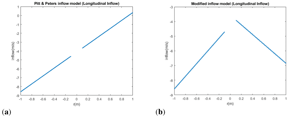
Figure 24 Comparison between original inflow model and modified inflow model based on CFD simulations:
(a) Original longitudinal inflow ( v i ( m/s ) ) MathType@MTEF@5@5@+= feaagKart1ev2aaatCvAUfeBSjuyZL2yd9gzLbvyNv2CaerbuLwBLn hiov2DGi1BTfMBaeXatLxBI9gBaerbd9wDYLwzYbItLDharqqtubsr 4rNCHbGeaGqk0dg9crFfpeea0xh9v8qiW7rqqrFfpeea0xe9Lq=Jc9 vqaqpepm0xbba9pwe9Q8fs0=yqaqpepae9pg0FirpepeKkFr0xfr=x fr=xb9adbaqaaeGaciGaaiaabeqaamaabaabaaGcbaWaaeWaaeaada WhcaqaaabaaaaaaaaapeGaamODa8aadaWgaaWcbaWdbiaadMgaa8aa beaaaOGaay51GaWaaeWaaeaapeGaamyBaiaac+cacaWGZbaapaGaay jkaiaawMcaaaGaayjkaiaawMcaaaaa@4200@ (b) Modified longitudinal inflow ( v i ( m/s ) ) MathType@MTEF@5@5@+= feaagKart1ev2aaatCvAUfeBSjuyZL2yd9gzLbvyNv2CaerbuLwBLn hiov2DGi1BTfMBaeXatLxBI9gBaerbd9wDYLwzYbItLDharqqtubsr 4rNCHbGeaGqk0dg9crFfpeea0xh9v8qiW7rqqrFfpeea0xe9Lq=Jc9 vqaqpepm0xbba9pwe9Q8fs0=yqaqpepae9pg0FirpepeKkFr0xfr=x fr=xb9adbaqaaeGaciGaaiaabeqaamaabaabaaGcbaWaaeWaaeaada WhcaqaaabaaaaaaaaapeGaamODa8aadaWgaaWcbaWdbiaadMgaa8aa beaaaOGaay51GaWaaeWaaeaapeGaamyBaiaac+cacaWGZbaapaGaay jkaiaawMcaaaGaayjkaiaawMcaaaaa@4200@ .

The estimation of the inflow affects the predictions having a bigger impact on the pitch optimization than on chord because the pitch is used to set the airfoils at maximum aerodynamic efficiency whereas the chord optimization is linked with profile drag and lift generation by available surface. Regarding to tip/hub losses, by contrast to hovering where upwash was observed near the tip. At these inflows though the downwash is reduced, the flow is far from changing its direction. This can be related with the presence of a lighter effect of tip vortexes. To check if this could have a substantial impact on the model, some modifications were performed. First, the tip/hub losses were removed, meaning that, it is assumed that the tip/hub sections can generate lift. Moreover, the linear models were modified to try to estimate inflows more like the predicted with the simulations. The modification of the inflow model was done with some simple changes. Figures 25 & 26 shows the comparison between original and modified models.
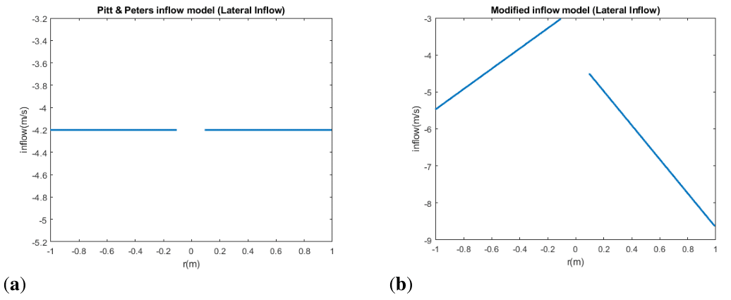
Figure 25 Comparison between original inflow model and modified inflow model based on CFD simulations:
(a) Original lateral inflow ( v i ( m/s ) ) MathType@MTEF@5@5@+= feaagKart1ev2aaatCvAUfeBSjuyZL2yd9gzLbvyNv2CaerbuLwBLn hiov2DGi1BTfMBaeXatLxBI9gBaerbd9wDYLwzYbItLDharqqtubsr 4rNCHbGeaGqk0dg9crFfpeea0xh9v8qiW7rqqrFfpeea0xe9Lq=Jc9 vqaqpepm0xbba9pwe9Q8fs0=yqaqpepae9pg0FirpepeKkFr0xfr=x fr=xb9adbaqaaeGaciGaaiaabeqaamaabaabaaGcbaWaaeWaaeaada WhcaqaaabaaaaaaaaapeGaamODa8aadaWgaaWcbaWdbiaadMgaa8aa beaaaOGaay51GaWaaeWaaeaapeGaamyBaiaac+cacaWGZbaapaGaay jkaiaawMcaaaGaayjkaiaawMcaaaaa@4200@ . (b) Modified lateral inflow ( v i ( m/s ) ) MathType@MTEF@5@5@+= feaagKart1ev2aaatCvAUfeBSjuyZL2yd9gzLbvyNv2CaerbuLwBLn hiov2DGi1BTfMBaeXatLxBI9gBaerbd9wDYLwzYbItLDharqqtubsr 4rNCHbGeaGqk0dg9crFfpeea0xh9v8qiW7rqqrFfpeea0xe9Lq=Jc9 vqaqpepm0xbba9pwe9Q8fs0=yqaqpepae9pg0FirpepeKkFr0xfr=x fr=xb9adbaqaaeGaciGaaiaabeqaamaabaabaaGcbaWaaeWaaeaada WhcaqaaabaaaaaaaaapeGaamODa8aadaWgaaWcbaWdbiaadMgaa8aa beaaaOGaay51GaWaaeWaaeaapeGaamyBaiaac+cacaWGZbaapaGaay jkaiaawMcaaaGaayjkaiaawMcaaaaa@4200@ .

Figure 26 Isolated optimizations of chord and twist for forward flight at 10 m/s with the modified model
(a) Optimal chord distributions. (b) Optimal twist distributions.

  1. Firstly, since a certain degree of symmetry is observed with respect to the azimuth position, the absolute value of the azimuth angle is considered in the equation 11.
  2. Secondly, lateral, and horizontal inflow is similar than. Pitt & Peters model assumes constant inflow for lateral inflow, Equation 11, however, for approximating the simulations, it is used the longitudinal inflow coefficient ( k x ) MathType@MTEF@5@5@+= feaagKart1ev2aaatCvAUfeBSjuyZL2yd9gzLbvyNv2CaerbuLwBLn hiov2DGi1BTfMBaeXatLxBI9gBaerbd9wDYLwzYbItLDharqqtubsr 4rNCHbGeaGqk0dg9crFfpeea0xh9v8qiW7rqqrFfpeea0xe9Lq=Jc9 vqaqpepm0xbba9pwe9Q8fs0=yqaqpepae9pg0FirpepeKkFr0xfr=x fr=xb9adbaqaaeGaciGaaiaabeqaamaabaabaaGcbaWaaeWaaeaaqa aaaaaaaaWdbiaadUgapaWaaSbaaSqaa8qacaWG4baapaqabaaakiaa wIcacaGLPaaaaaa@3C0B@ .
  3. Finally, since both blades showed different initial inflow values but only slightly different slopes, it is applied a sigmoid function between the opposite azimuth angles. Smoothly reducing the initial inflow and varying slightly the slope.

After that, optimization was run again for the case of V f =10m/s MathType@MTEF@5@5@+= feaagKart1ev2aaatCvAUfeBSjuyZL2yd9gzLbvyNv2CaerbuLwBLn hiov2DGi1BTfMBaeXatLxBI9gBaerbd9wDYLwzYbItLDharqqtubsr 4rNCHbGeaGqk0dg9crFfpeea0xh9v8qiW7rqqrFfpeea0xe9Lq=Jc9 vqaqpepm0xbba9pwe9Q8fs0=yqaqpepae9pg0FirpepeKkFr0xfr=x fr=xb9adbaqaaeGaciGaaiaabeqaamaabaabaaGcbaaeaaaaaaaaa8 qacaWGwbWdamaaBaaaleaapeGaamOzaaWdaeqaaOWdbiabg2da9iaa igdacaaIWaGaamyBaiaac+cacaWGZbaaaa@3F83@ . Regarding to chord optimization, no significant changes were found with the linear and quadratic distributions, which still are worse than the baseline. Two linear segment distributions were the same than the obtained in the first optimization, Table 11, and Figure 13. Regarding to Bézier, almost no changes are observed, results are in Table 28.

Vf(m/s)

Croot

tap

r3

y4

r5

y6

P(W)

10

0.01

1

0.4

0.04

0.72

0.04

62.9368

Table 28 Bézier chord distribution parameters and power requirements, modified model optimizations at forward flight

With respects to twist, some interesting results were achieved, new distributions differ to the previous from the original model. Parameters are gathered in Table 29 whereas Figure 27 shows the distributions.

Case

θroot

θtip /a1/ slp

r3 /slp2

y4 / rperc

r5

y6

P(W)

Lin. Twist

0.3601

- / - / -0.2211

- / -

- / -

-

-

60.6125

Quad. Twist

0.4363

- / 0.253 / -

- / -

- / -

-

-

60.7312

2 Lin. Twist

0.4061

- / - / -0.1066

- / -0.1359

- / 0.3324

-

-

60.5457

Béz. Twist

0.4316

0.1714 / - / -

0.3635 / -

0.3026 / -

0.7223

0.2050

60.4866

Table 29 Twist distributions parameters and power requirements, modified model optimizations at forward flight
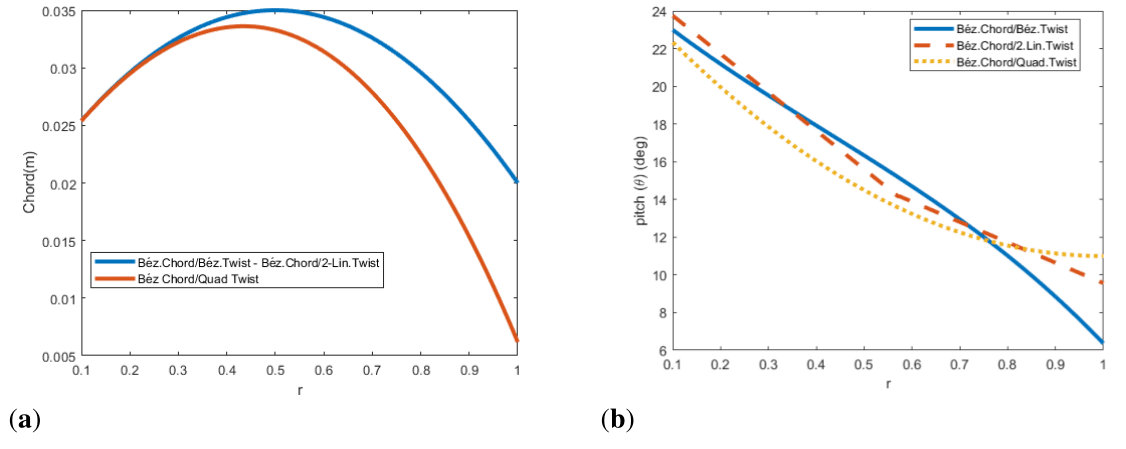
Figure 27 Combined optimizations of chord and twist distributions for forward flight at 10 m/s
(a) Optimal chord distributions. (b) Optimal twist distributions.

The new twist rate in all distributions is more moderate and the airfoils near the tip are set with bigger pitch angles. Apart from that, the spline distribution shows a quite linear behavior.

Moreover, it was performed the dual optimization of chord and twist. Whose results are shown in Tables 30 & 31. General tendencies analyzed before are observed again, negative twist enhances the performance, twist implementation helps setting the airfoils at angle of attacks for which aerodynamic efficiency is high, as it approaches to the tip, the inflow angle ( ϕ=atan( U P / U T ) ) MathType@MTEF@5@5@+= feaagKart1ev2aqatCvAUfeBSjuyZL2yd9gzLbvyNv2CaerbuLwBLn hiov2DGi1BTfMBaeXatLxBI9gBaerbd9wDYLwzYbItLDharqqtubsr 4rNCHbGeaGqk0dg9crFfpeea0xh9v8qiW7rqqrFfpeea0xe9Lq=Jc9 vqaqpepm0xbba9pwe9Q8fs0=yqaqpepae9pg0FirpepeKkFr0xfr=x fr=xb9adbaqaaeGaciGaaiaabeqaamaabaabaaGcbaaeaaaaaaaaa8 qadaqadaqaaiabew9aMjabg2da9iaabggacaqG0bGaaeyyaiaab6ga caGGOaGaamyva8aadaWgaaWcbaWdbiaadcfaa8aabeaak8qacaGGVa Gaamyva8aadaWgaaWcbaWdbiaadsfaa8aabeaak8qacaGGPaaacaGL OaGaayzkaaaaaa@468F@ decreases as a consequence of the higher tangential speed that increases faster than the induced speed. Hence, the required pitch for keeping a moderate angle of attack is smaller, as a result of this, the same thrust is generated with lower rotational required speed than the baseline, which affects the drag, as reflected in Table 5 for hovering and by Figure 28(a). With respects to chord, it is increased in middle sections of the blades and reduce near the tips were drag is bigger. As mentioned during the introduction, the benefit of the larger chords is linked with the higher Reynolds regime over the blades. Particularly, thick airfoils with non-ideal designed for operating at these regimes, such as the used NACA 0012, increased their efficiency rapidly even with small variations of the Reynolds regime. Moreover, despite this effect cannot be considered since the data base is fixed, the chord variation would have an impact on the thickness ratio of the airfoils, making them more slender bodies, which as stated by other researchers that did analyze the optimization of the airfoils,4 is interesting at low Reynolds regimes. Further justification and explanation of the optimal shapes would require a more thorough analysis, CFD simulations can also be used for studying the physics around the blades and can be used for studying the wake and checking distributions such as lift or pressure along the blade.

Case

Croot

tap

r3

y4

r5

y6

P(W)

Béz.Chord/Béz.Twist

0.0200

1.0000

0.2317

0.0400

0.7783

0.0400

57.31

Béz Chord/2 Lin Twist

0.0200

1.0000

0.4491

0.0500

0.7197

0.0130

58.43

Béz Chord/Quad Twist

0.0200

0.3091

0.4323

0.0400

0.7974

0.0400

57.85

Table 30 Chord distribution parameters and power requirements, modified model combined twist and chord optimizations at forward flight

Case

θroot

θtip /a1/ slp

r3 /slp2

y4 / rperc

r5

y6

P(W)

Béz.Chord/Béz.Twist

0.4363

0.1111 / - / -

0.3490 / -

0.3125 / -

0.7783

0.2656

57.31

Béz.Chord/2 Lin. Twist

0.4145

- / - / -0.1673

- / -0.0803

- / 0.5727

-

-

58.43

Béz.Chord/Quad. Twist

0.4362

- / 0.2443 / -

- / -

-

-

-

57.85

Table 31 Twist distribution parameters and power requirements, modified model combined twist and chord optimizations at forward flight

These new geometries were simulated in CFD and the estimations for the baseline were compared with the new model predictions. Figure 28 shows the comparative between the simulations and the estimations form the modified model.
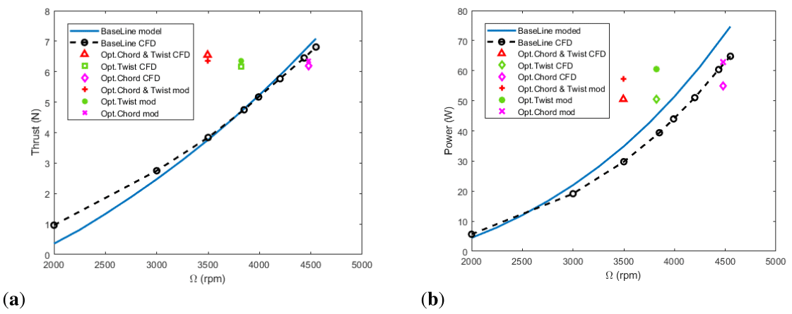
Figure 28 Comparison between modified model estimations and CFD simulations of the baseline rotor and some optimal rotors at forward flight
(a) Thrust (N) versus rotational speed ( Ω( rpm ) ) MathType@MTEF@5@5@+= feaagKart1ev2aqatCvAUfeBSjuyZL2yd9gzLbvyNv2CaerbuLwBLn hiov2DGi1BTfMBaeXatLxBI9gBaerbd9wDYLwzYbItLDharqqtubsr 4rNCHbGeaGqk0dg9crFfpeea0xh9v8qiW7rqqrFfpeea0xe9Lq=Jc9 vqaqpepm0xbba9pwe9Q8fs0=yqaqpepae9pg0FirpepeKkFr0xfr=x fr=xb9adbaqaaeGaciGaaiaabeqaamaabaabaaGcbaWaaeWaaeaaju gibabaaaaaaaaapeGaaeyQdOWdamaabmaabaqcLbsapeGaaeOCaiaa bchacaqGTbaak8aacaGLOaGaayzkaaaacaGLOaGaayzkaaaaaa@40AB@ . (b) Power (W) versus rotational speed ( Ω( rpm ) ) MathType@MTEF@5@5@+= feaagKart1ev2aqatCvAUfeBSjuyZL2yd9gzLbvyNv2CaerbuLwBLn hiov2DGi1BTfMBaeXatLxBI9gBaerbd9wDYLwzYbItLDharqqtubsr 4rNCHbGeaGqk0dg9crFfpeea0xh9v8qiW7rqqrFfpeea0xe9Lq=Jc9 vqaqpepm0xbba9pwe9Q8fs0=yqaqpepae9pg0FirpepeKkFr0xfr=x fr=xb9adbaqaaeGaciGaaiaabeqaamaabaabaaGcbaWaaeWaaeaaju gibabaaaaaaaaapeGaaeyQdOWdamaabmaabaqcLbsapeGaaeOCaiaa bchacaqGTbaak8aacaGLOaGaayzkaaaacaGLOaGaayzkaaaaaa@40AB@ .

It is observed that the overestimation of thrust has been reduced. Furthermore, opposite to previous optimization, the new geometries enhance the performance of the baseline rotor, as estimated by the model. The Table 32 shows the estimations of power of each of the geometries and the power reduction with respect to the baseline as well as the estimated pilot input for reaching that performance.

Optim.Rotor // BL

T (N)

Ω (rpm)

P (W)

ΔP(%)

Béz.Chord // BL

6.35 // 6.35

4478 // 4347

62.93 // 65.1

-3.33

Béz.Chord & Twist // BL

6.35 // 6.35

3495 // 4467

57.32 // 65.1

-11.95

Béz.Twist // BL

6.35 // 6.35

3822 // 4334

60.49 // 65.1

-7.08

Table 32 Power requirements comparison of different rotors Estimations from the modified forward flight model

New model predicts improvements from the baseline geometry, however, despite it happened before, the power reductions are more conservative, and they seem less optimistic than the previous ones. Table 33 shows the same results but obtained from CFD simulations.

Optim.Rotor // BL

T (N)

Ω (rpm)

P (W)

ΔP(%)

Béz. Chord // BL

6.197 // 6.197

4478 // 4347

55.014 // 56.82

-3.18

Béz. Chord/Twist // BL

6.55 // 6.55

3495 // 4467

50.51 // 61.58

-17.97

Béz. Twist // BL

6.1741 // 6.1741

3822 // 4334

50.58 // 56.49

-10.46

Table 33 Power requirements comparison of different rotors Estimations from the CFD simulations at forward flight

Clearly, the modifications in the model provide more accurate results. The power reductions estimated are confirmed with the CFD simulations.

Conclusion

The present study assessed the feasibility of developing low-fidelity models for small-scale rotors as a cost-effective alternative to more expensive tools. The model based on BEMT for hovering, implemented in MATLAB using XFOIL for airfoil properties, showed good agreement with CFD simulations. The second model for forward flight, however, overestimated thrust generation and power reduction of variable pitch rotors. The proposed chord optimizations improved baseline performance, but variable pitch benefits were not reflected in the simulations. Simulations showed non-uniform inflows contradicting linear theoretical models. Adjusting the inflow reduced thrust overestimation but continued to predict lower power demands with decreased pitch near tips. 3D losses functions direct applicability for forward flight was uncertain, hence, they were removed from the model. New optimized geometries resulted in different pitch distributions without affecting chord distributions. CFD simulations agree with

would be the impact on the thickness ratio of the airfoils. Optimizations predicted power reductions of 3−4% for chord, 7−11% for twist, and up to 17% for combined distributions.

Despite CFD is a higher fidelity tool than theoretical models, it would be interesting to perform wind tunnel tests for checking the results. the new model predictions.

In summary, linear inflow assumptions were invalidated by CFD results, impacting rotor performance predictions. Hub/tip losses models' applicability in forward flight remains uncertain. Variable chord and pitch distributions offer potential improvements in small-scale rotor designs. As it happens for large scale rotors, negative twist implementation shows promising results for reducing power demands. The variation of pitch along the blade try to set all the airfoils sections at angles of attack with better aerodynamic efficiency. In terms of chord distributions, by contrast to large scale rotors, for which tapered blades are common, for small scale rotors seems interesting a concave shape. Increasing the chord implies bigger Reynolds over the blade, which enhances airfoil aerodynamic efficiency due to the low Reynolds regime, in which small changes have an important impact on the lift/drag ratio, another positive effect that cannot be quantified Moreover, CFD simulations were performed focusing on validating the models, but they can also be used as a tool for analyzing thoroughly the physics and impact of the geometrical changes on the flow over the blades. Additionally, the created models can be used for analyzing other sizes of rotors for heavier vehicles apart from studying other parameters such as the number of blades as well as they can be used as a base for implementing new parametrical effects considerations such as tip shapes effects.

Acknowledgments

The authors acknowledge the support of Fundação para a Ciência e a Tecnologia (FCT), through IDMEC, under LAETA, with grant number (UIDB/50022/2020).

Conflicts of interest

The authors declare that there is no conflict of interest.

References

  1. Cagnato R. Study on the effect of curvature on the aerodynamic properties of drone rotor blades. Master Thesis, Master of Science Degree in Aerospace Engineering-Instituto Técnico Superior, Universidad de Lisboa; 2020.
  2. Caceres Andrade CA. Design of an aerodynamic profile for low Reynolds numbers using computational tools. Final Degree Project, Degree in Mechanical Engineering-Universidad de Pamplona; Colombia: 2021.
  3. Walsh JL. Performance optimization of helicopter rotor blades. Proceedings of the Air Force/NASA Symposium on Recent Advances in Multi-Disciplinary Analyses and Optimization; 1990 September 24-26; San Francisco, CA, United States: NASA; 1991.
  4. Bohorquez F. Rotor hover performance and system design of an efficient coaxial rotary wing micro air vehicle. Doctoral dissertation, College Park: University of Maryland; 2007.
  5. Winslow J, Otsuka H, Govindarajan B, et al. Basic understanding of airfoil characteristics at low Reynolds Numbers (104–105). J Aircraft. 2017;55:1050–1061.
  6. Wiebe J. Development of a simulation and optimization framework for improved aerodynamic performance of R/C helicopter rotor blades. Master Thesis, Master of Applied Science in Aerospace Engineering, Ottawa: Carleton Institute for Mechanical and Aerospace Engineering; 2015.
  7. Kodchaniphaphong C, Pukrushpan J, Klumpol C. Investigating and analyzing the potential for regenerating excess energy in a helicopter UAV. Drones. 2023;7(10):643.
  8. Fernandes de Vasconcelos CH. Aerodynamic effect of different drone blade tip shapes. Master thesis, Master of Science Degree in Aerospace Engineering-Instituto Superior Técnico, University of Lisbon; 2023.
  9. The MathWorks Inc. MATLAB version: 9.13.0 (R2022b), Natick, Massachusetts: 2022.
  10. Drela M. XFOIL version 6.99, Cambridge, Massachusetts: Massachusetts Institute of Technology; 2000.
  11. Ansys Inc. Ansys fluent version 2021 R2, Canonsburg, Pennsylvania: 2021.
  12. Pelletier A, Mueller TJ. Low Reynolds Number aerodynamics of low-aspect-ratio, thin/flat/cambered-plate wings. J Aircraft. 2000;37:825–832.
  13. Ohtake T, Nakae Y, Motohashi T. Nonlinearity of the aerodynamic characteristics of NACA0012 Aerofoil at Low Reynolds Numbers. J Japan Soc Aeronaut Space Sci. 2007;55(644):439–445.
  14. Ahmad M, Li B. A comparative analysis of turbulence models in FLUENT for high-lift airfoils at low Reynolds Number. In: International Conference on Unmanned Aircraft Systems (ICUAS); 2022. p. 779–786.
  15. Drela M. XFOIL: An analysis and design system for low Reynolds Number airfoils. In: Conference on Low Reynolds Number Airfoil Aerodynamics; 1989 June 5-7; University of Notre Dame; Indiana, USA: 1989.
  16. Leishman JG. Principles of helicopter aerodynamics. 2nd ed. In: Cambridge Aerospace Series. 32 Avenue of the Americas, New York, NY 10013-2473, USA: Cambridge University Press; 2006. p. 60–273.
  17. Theys B, De Schutter J. Forward flight tests of a quadcopter unmanned aerial vehicle with various spherical body diameters. International Journal of Micro Air Vehicles. 2020;12.
  18. Zabotto Chiusoli R. Experimental study of modifications of drone propeller blades for noise reduction and performance. Master thesis, Master of Science Degree in Aerospace Engineering- Instituto Superior Técnico, University of Lisbon; 2023.
  19. Kolaei A, Barcelos D, Bramesfeld G. Experimental analysis of a small-scale rotor at various inflow angles. Int J Aerospace Eng. 2018;2560370.
  20. The MathWorks Inc. MATLAB global optimization toolbox user’s guide R2024, Natick, Massachusetts: 2024.
  21. Conn AR, Gould N, Toint PL. A globally convergent augmented lagrangian barrier algorithm for optimization with general inequality constraints and simple bounds. Mathematics of Computation. 1997;66(217):261–288.
  22. K-Omega Turbulence Models; SimScale.
  23. Nathanael JC, Wang JC, Low KH. Numerical studies on modelling the near and far field wake vortex of a quadrotor in forward flight. Proceedings of the Institution of Mechanical Engineers, Part G: Journal of Aerospace Engineering. 2022;236(6):1166–1183.
Creative Commons Attribution License

©2024 Ortiz, et al. This is an open access article distributed under the terms of the, which permits unrestricted use, distribution, and build upon your work non-commercially.