Weirs are the common structure uses in the most of water engineering projects such as Hydropower systems, irrigation and drainage networks and sewage networks. Side weir has many possible uses in the hydraulic engineering field and also has been investigated as an important structure in hydro systems. In this paper, predicting the side weir discharge coefficient was considered by using the empirical formulas, multi–layer perceptron (MLP) and radial basis function (RBF) neural as a delegate of artificial neural network models. The results indicate that the Emiroglu formula by the correlation coefficient (0.65) and root mean square error (0.03) is accurate among the empirical formulas. Evaluating the performance of the MLP model by the correlation coefficient (0.89) and root mean square error (0.067) and RBF model by the correlation coefficient (0.71) and root mean square error (0.08) show are more accurate in compare to the empirical formulas. When the MLP model was more accurate than RBF models.

Keywords: weirs, discharge coefficient, empirical formulas, multi–layer Perceptron, performance

Modeling of Hydraulic structures has received much attention in recent years due to these effect on the increasing the hydro system performance.¹ Weirs are the common structure which uses in the most of water engineering projects such as hydropower systems, irrigation and drainage networks and sewage networks. Side weir has many possible uses in the hydraulic engineering field and has also been investigated as an important structure in hydro systems.^2,3 Side weir is a hydraulic structure placed on the side of the channel and sometime uses as water surface controller structure in the dam an irrigation projects. Whereas the main duty of the side weir is removing the excess flow from the hydro systems.^4,5 Figure 1 shows an schematic scheme of the side weir in subcritical flow condition. Study on the side weir hydraulics conducted by the physical and numerical approaches. In the physical studies field, researchers tried to improve the performance of side weir by proposing the various shape for the crest of the side weir and compared this performance with a rectangular shape as a standard form for side weir. In this regard, labyrinth, oblique, semi–elliptical, curved plan–form and trapezoidal sharp and broad–crested can be mentioned.^5–13 Researchers who conducted an experimental study on the hydraulic side weir proposed empirical equations for calculating the side weir discharge coefficient. A summary of the most famous empirical formulas gives in the Table 1. In the numerical modeling field in addition to solving the government hydraulically equations by numerical approaches and such as Runge Kutta Method, the computational fluid dynamic (CFD) techniques have been used to simulate the flow over side weir. Numerical solving the government equations leads to define the hydraulic parameters such as water surface profile, distribution of velocity and pressure and flow pattern.^14,15 Another way as numerical modeling are related to use the artificial neural network (ANN) models for predicting the hydraulic properties of side weir such as discharge coefficient. In this regard, the Multilayer Preceptor (MLP) neural network, Adaptive Neuro–Fuzzy Inference System (ANFIS) was used by researchers. Developing the ANN models is based on the dataset. It means that to predict the hydraulic phenomenon by neural network techniques, the parameters which are an influence on the phenomenon should be measured at the previous. The ANN models can use as standalone and also applied as a participant of the numerical methods in numerical simulation to increase the accuracy of the numerical modeling. The results of using the mentioned neural network models indicate that ANN models are more accurate.^10,15–19 In this research, the radial basis function (RBF) neural network which has high performance in pattern recognition and image processing is developed for predicting the side weir discharge coefficient and its performance is compared with empirical formula and multilayer perceptron neural network as common ANN model which uses by most of the researchers.

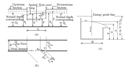
Figure 1 Sketch of side weir structure in subcritical flow condition.

The side weir discharge coefficient is a function of hydraulic characteristics and geometry of the side weir and canal. Most hydraulic and geometry parameters as shows in the Figure 1. Defining the effect of each influence parameter needs to conduct the experiment in condition which the other parameters are constant. Researchers try to reduce the number of experiments by using the dimensional analysis techniques such as Buckingham theory. Using the analysis techniques leads to derive dimensionless parameters. As mentioned in the previous section, the side weir discharge coefficient $\left(\text{C}{\text{d}}_{\text{sw}}\right)$  is a function of hydraulic and geometry properties so the general form of the $\left(\text{C}{\text{d}}_{\text{sw}}\right)$ gives in equation (1).

$\text{C}{\text{d}}_{\text{sw}}\text{=f}\left({\text{v}}_{\text{1}}\text{,L,b,}{\text{h}}_{\text{1}}\text{,P,ψ,}{\text{s}}_{\text{0}}\right)$                                             (1)

Where;
b: is the width of channel,
${\text{h}}_{\text{i}}$ : flow depth in the main channel,
${\text{v}}_{\text{i}}$ : mean velocity of the flow at upstream end of side weir,
L: length of side weir,
${\text{s}}_{\text{0}}$ : slope of main channel bed,
g: acceleration due to gravity,
P: weir height and
$\Psi$ : deviation angle of flow.

Dimensionless parameters are derived by using the Buckingham theory as equation (2). El–Khashab et al.²⁰ state that the L/b includes the effect of flow deviation angle.

$\text{C}{\text{d}}_{\text{sw}}\text{=}{\text{f}}_{\text{2}}\left(\text{F}{\text{r}}_{\text{1}}\text{,}\frac{\text{L}}{\text{b}}\text{,}\frac{\text{L}}{{\text{h}}_{\text{1}}}\text{,}\frac{\text{P}}{{\text{h}}_{\text{1}}}\right)$                 (2)

In equation (2) the $\text{F}{\text{r}}_{\text{1}}$ is the Froude number. As present in the Table 1 most of the empirical formulas used the dimensionless parameters. Using the dimensionless parameters in ANN model preparation leads to create an optimal structure during the development process. Developing the MLP and RBF models as similar to other neural network models is based on data set. To this purpose 477 data set related to the side weir discharge coefficient which published in the creditable journals was collected. Some of the resources that were used for data derivation are given as follows.^4,11,21–23 The range of the collected data is given in Table 2.

Multilayer Perceptron (MLP) neural network
ANN is a nonlinear mathematical model that can simulate arbitrarily complex nonlinear processes that relate the inputs and outputs of any system. In many complex mathematical problems that lead to solving complex nonlinear equations, Multilayer Perceptron networks are common types of ANN that are widely used by researches . To use MLP model, the definition of appropriate functions, weights and bias should be considered. Due to the nature of the problem, different activity functions in neurons can be used. An ANN maybe has one or more hidden layers. Figure 2 demonstrates a three–layer neural network consisting of inputs layer, hidden layer (layers) and outputs layer. As shown in Figure 2. W is the weight and ${\text{b}}_{\text{i}}$ is the bias for each neuron. Weight and biases' values will be assigned progressively and corrected during training process comparing the predicted outputs with known outputs. Such networks are often trained using back propagation algorithm. In the present study, ANN was trained by Liebenberg–Marquardt technique because this technique is more powerful and faster than the conventional gradient descent technique.^{24, 25}

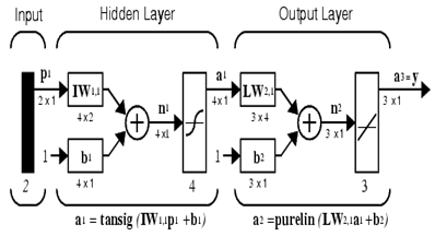
Figure 2 A three-layer ANN architecture.

Radial Basis Function (RBF) neural network
Radial Basis Function (RBF) Neural Network is a type of artificial neural networks which widely uses in image processing, pattern recognition, and nonlinear system modeling. The RBF model as shown in the Figure 3 consists of two layers, the first layer considered a hidden layer and the second layer as the output layer. The radial function is considered the transfer function for the neurons which are in the hidden layer and linear function as output layer transfer function. Designing the RBF neural network is based on the defining the center of these functions in other to the aim of RBF model training is mapping the input space to output space as. The transfer function of the RBF model is defined as equation (3).
$\text{f}\left(\text{ν}\right)\text{=}{\displaystyle \sum _{\text{i=1}}^n{\text{w}}_{\text{i}}\text{φ}}\left(\left|\left|\text{ν-}{\text{c}}_{\text{i}}\right|\right|\right)$                                                       (3)

Where
$\text{v}$ : is the input variable, is the weight coefficients,
$\text{φ}$ : is a Gaussian function which is the basic function that uses a kernel function in RBF model development and defines as equation (4).

$\text{φ}\left(\text{ν}\right)\text{=}{\text{e}}^{\left(\frac{\text{-}{\text{ν}}^{\text{2}}}{\text{2}{\sigma }^{\text{2}}}\right)}$                                      (4)

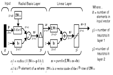
Figure 3 A RBF model structure.

The RBF model training usually is carried out by Gradient Descent approach. The aim of the RBF model is defining the value of the kernel function parameters and weights. The initial value of the weights is defined randomly. The error for each sample of the data set is calculated by using equation (5).

${\text{e}}_{\text{i}}\text{=}{\text{t}}_{\text{i}}\text{-}{\text{y}}_{\text{i}}\text{=}{\text{t}}_{\text{i}}\text{-}{\displaystyle \sum _{\text{j=1}}^{\text{N}}\text{w}}\text{φ}\left(\left|\left|{\text{ν}}_{\text{i}}\text{-}{\text{c}}_{\text{i}}\right|\right|\right)$           (5)

The error for the total input data set is calculated as equation (6).

$\text{E=}\frac{\text{1}}{\text{2}}{\displaystyle \sum _{\text{i=1}}^{\text{p}}{\left|{\text{e}}_{\text{i}}\right|}^{\text{2}}}$                   (6)

The EBF model is finished when the error of the RBF model for all the data set is lower than the threshold error which is defined by the designer.

The performance of empirical formulas, MLP and RBF models was assessed by the data collected that range of them gives in the Table 2. The accuracy of the empirical formulas and MLP and RBF models was assessed by statistical error indices such as correlation coefficient, Root Mean Square Error, Mean Square Error. It is noticeable that these indices provide an average value for error and doesn't give any information about error distribution, so It is advisable that in addition to calculating the indices error, the performance of these shows a figure between the measured values and calculated or predicted values. All the stages of the MLP and RBF models development were programmed in the environment of Matlab software.

The experimental formulas Results
The performance of the empirical formulas was evaluated for calculating the by using the data collection (Table 2) and results of them compared with the measured data. Table 3 presents the results of empirical formulas. As given in Table 3 most empirical formula hasn’t suitable performance. Based on the Table 2, the Emiroglu formula is accurate by correlation coefficient about 64%. The performance of the Emiroglu formula versus the measured data was plotted in Figure 4.

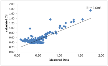
Figure 4 Results of the Emiroglu formula versus the measured data.

ANN models results

Developing the MLP and RBF models is based on the dataset. The dataset was divided in to two groups as training and testing data. Data selection for the ANN model training and the testing process carried out by random approach. Designing the ANN model structure is more based on the designer experience, but the investigator’s recommendation who conducted similar research is useful. Designing the ANN model is recommending the type of the neural network model, number of the hidden layer(s), number of the neurons in each layer, and defining the suitable transfer function for the neurons of hidden and output layers.

MLP models Results
The MLP model contains two layers; inputs and hidden layers. The hidden layer contains ten (10) neurons and transfer functions were tangent sigmoid (tansig). (Figure 5) The MLP model structure is shown in the Figure 6. The training of the MLP model was performed with levenberg_marquat technique. 70 percent of data set was used for training, 15 percent for validation and other (15 percent) was considered for testing the model. The performance of MLP model in each stage of development (Train, Validation, and Testing) is shown in the Figure 6, Figure 7, Figure 8 and to assess the performance of this model, error indices for each stage of preparation was calculated and presented in these figures. Figure 6, Figure 7, Figure 8 shows that the accuracy of the MLP model is suitable for prediction of the$\left(\text{C}{\text{d}}_{\text{sw}}\right)$ . In addition to calculation standard error indices, the error distribution for the all data which were used for training, validation, and testing was also plotted. To evaluate the error density the error histogram was plotted. As seems from the histogram the distribution of the error is normal and more concentrated around the zeros.

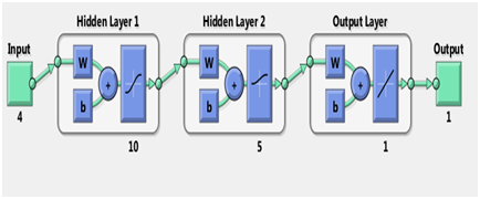
Figure 5 The structure of the MLP model.

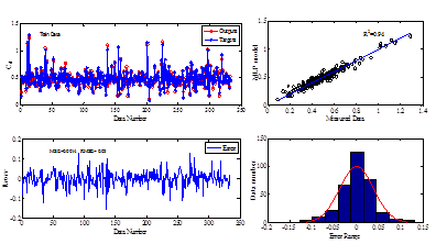
Figure 6 The performance of the MLP model during the training stage.

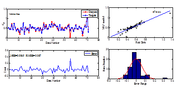
Figure 7 The performance of the MLP model during the validation stage.

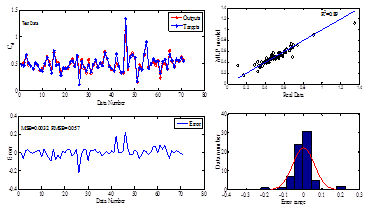
Figure 8 The performance of the MLP model during the validation stage.

RBF models results
To assess the accuracy of the RBF model for prediction of the $\left(\text{C}{\text{d}}_{\text{sw}}\right)$ and also to comparing its performance with MLP model tried to hold similar conditions for model development. In other to tried to hold a similar number of the training, validation and testing data set. In addition, tried to similar hold the number of the neurons in the input layer. The architect of the RBF model is shown in the Figure 9. As show n in the Figure 9 the input layer neurons was considered as equal to the MLP model input later. The performance of the RBF model during the training, validation and testing model is shown in the Figure 10, Figure 11, Figure 12. As shown from these figures, the performance of the RBF model to predict the $\left(\text{C}{\text{d}}_{\text{sw}}\right)$ is not so suitable. Comparing the performance of the RBF model with MLP model in training, validation and testing stages shows that the MLP model is more accurate.

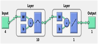
Figure 9 The architect of the RBF model.

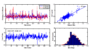
Figure 10 The performance of the RBF model during the training stage.

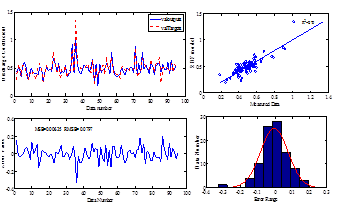
Figure 11 The performance of the RBF model during the validation stage.

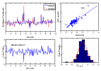
Figure 12 The performance of the MLP model during the validation stage.

In this study, the side weir discharge coefficient $\left(\text{C}{\text{d}}_{\text{sw}}\right)$ was calculated and predicted by empirical formulas and radial basis function (RBF) neural network and multilayer perceptron (MLP) neural network. The results of this study indicate that the Emiroglu formula is accurate among the empirical formula. To achieve more accuracy in $\left(\text{C}{\text{d}}_{\text{sw}}\right)$ prediction, the MLP model and RBF model was developed, to prepare the MLP and RBF models the about 477 dataset related the $\left(\text{C}{\text{d}}_{\text{sw}}\right)$ was collected. The result of the suitable the performance of the MLP shows that the MLP model has assessing performance to predict the$\left(\text{C}{\text{d}}_{\text{sw}}\right)$ . The results of the RBF model development indicated the accuracy of this model is a little better than the empirical formals. In overall, the performance of the MLP model is much more than the RBF and empirical formulas.

None.

The author declines there is no conflict of interest.

1. Ettema R. Hydraulic Modeling: Concepts and Practice. ASCE. 2000: 390 p.
2. Laycock A. Irrigation Systems: Design, Planning and Construction. CABI. 2007: 285 p.
3. Te Chow V. Open–channel Hydraulics. Blackburn Press. Japan; 2009.
4. Bagheri S, Kabiri–Samani AR, Heidarpour M. Discharge coefficient of rectangular sharp–crested side weirs, Part I: Traditional weir equation. Flow Measurement and Instrumentation. 2014;35:109–115.
5. Haddadi H, Rahimpour M. A discharge coefficient for a trapezoidal broad–crested side weir in subcritical flow. Flow Measurement and Instrumentation. 2012;26:63–67.
6. Borghei SM, Parvaneh A. Discharge characteristics of a modified oblique side weir in subcritical flow. Flow Measurement and Instrumentation. 2011;22(5):370–376.
7. Cheong H. Discharge Coefficient of Lateral Diversion from Trapezoidal Channel. Journal of Irrigation and Drainage Engineering. 1991;117(4):461–475.
8. Coşar A, Agaccioglu H. Discharge Coefficient of a Triangular Side–Weir Located on a Curved Channel. Journal of Irrigation and Drainage Engineering. 2004;130(5):410–423.
9. Emiroglu M, Kaya N. Discharge Coefficient for Trapezoidal Labyrinth Side Weir in Subcritical Flow. Water Resources Management. 2011;25(3):1037–1058.
10. Emiroglu M, Kisi O. Prediction of Discharge Coefficient for Trapezoidal Labyrinth Side Weir Using a Neuro–Fuzzy Approach. Water Resources Management. 2013;27(5):1473–1488.
11. Emiroglu ME, Agaccioglu H, Kaya N. Discharging capacity of rectangular side weirs in straight open channels. Flow Measurement and Instrumentation. 2011;22(4):319–330.
12. Jalili M, Borghei S. Discussion: Discharge Coefficient of Rectangular Side Weirs. Journal of Irrigation and Drainage Engineering. 1996;122(2):132–132.
13. Kaya N, Emiroglu ME, Agaccioglu H. Discharge coefficient of a semi–elliptical side weir in subcritical flow. Flow Measurement and Instrumentation. 2011;22(1):25–32.
14. Mohammed AY. Numerical analysis of flow over side weir. Journal of King Saud University – Engineering Sciences. 2015;27(1);37–42.
15. Parsaie A, Haghiabi A. The Effect of Predicting Discharge Coefficient by Neural Network on Increasing the Numerical Modeling Accuracy of Flow Over Side Weir. Water Resources Management. 2015;29(4):973–985.
16. Bilhan O, Emin Emiroglu M, Kisi O. Application of two different neural network techniques to lateral outflow over rectangular side weirs located on a straight channel. Advances in Engineering Software. 2010;41(6):831–837.
17. Bilhan O, Emiroglu ME, Kisi O. Use of artificial neural networks for prediction of discharge coefficient of triangular labyrinth side weir in curved channels. Advances in Engineering Software. 2011;42(4):208–214.
18. Emiroglu ME, Bilhan O, Kisi O. Neural networks for estimation of discharge capacity of triangular labyrinth side–weir located on a straight channel. Expert Systems with Applications. 2011;38(1):867–874.
19. Kisi O. Prediction of lateral outflow over triangular labyrinth side weirs under subcritical conditions using soft computing approaches. Expert Systems with Applications. 2012;39(3):3454–3460.
20. El–Khashab A, Smith KV. Experimental investigation of flow over side weirs. Journal of the Hydraulics Division. 1976;102(9):1255–1268.
21. Singh R, Manivannan D, Satyanarayana T. Discharge Coefficient of Rectangular Side Weirs. Journal of Irrigation and Drainage Engineering. 1994;120(4):814–819.
22. Borghei S, Jalili M, Ghodsian M. Discharge Coefficient for Sharp–Crested Side Weir in Subcritical Flow. Journal of Hydraulic Engineering. 1999;125(10):1051–1056.
23. Subramanya K, Awasthy SC. Spatially varied flow over side–weirs. Journal of the Hydraulics Division.1972;98(1):1–10.
24. Aleksander I, Morton H. An Introduction to Neural Computing. Internat. Thomson Computer Press; 1995.
25. Sivanandam SN, Deepa SN. Introduction to Neural Networks Using Mat lab. Tata McGraw–Hill, USA; 2006.