The objective of the current study is to provide a further example which shows that a non-traditional mathematical modeling method can be advantageously used for mathematical modeling in pharmacokinetics. The current study is a companion piece of the earlier study by Belanger et al.¹, published in April 1987 issue of the Journal of Pharmacokinetics and Biopharmaceutics, therefore the data published in the study cited here was used. As stated above, an advanced modeling method based on the theory of dynamic systems was employed. Mathematical modeling was performed using the program named CTDB, described in the study by Dedík et al. ², published in September issue of the Journal Diabetes Research and Clinical Practice. All mathematical models developed, successfully described the pharmacokinetic behavior of acetaminophen in adult male Sprague-Dawley rats investigated in the experiment described in the study by Belanger et al. ¹. The modeling method used in the current study is universal, comprehensive, and flexible. Therefore, it can be used to develop mathematical models not only in the field of pharmacokinetics but also in several other scientific and practical fields.

Keywords: pharmacokinetics, temporal variations, mathematical model, dynamic system, biopharmaceutics, distribution

ADME, absorption/distribution/metabolism/elimination; AIC, akaike information criterion; CTDB, clinical trials database

In pharmacokinetics, mathematical modeling is usually preformed using only a measured concentration time profile of a drug administered in plasma and/or in blood. In contrast, if a modeling method based on the theory of dynamic systems is used in pharmacokinetics, then the mathematical modeling is performed using both: a mathematically described drug administration and a mathematically described body response to an administered drug. The main advantage of a modeling method based on the theory of dynamic systems is that, under the condition that the pharmacokinetic behavior of an administered drug is linear then an identical model structure can be used for e.g. an intravenous administration of a drug, an oral administration of a drug, an intramuscular administration of a drug and so on. An explanatory picture and some of full texts journal articles, written in a tutorial way, are available completely free of costs at: http://www.uef.sav.sk/durisova.htm and http://www.uef.sav.sk/advanced.htm.

Acetaminophen (N-4(hydroxyphenyl) acetamide) is an anti-inflammatory drug with few side effects. It is frequently used in analgesic and anti-pyretic treatment.^1,3–5 Time-dependent variations in organ extraction ratios of acetaminophen in rats were investigated in the experiment described in the study by Belander et al. published in April issue of the Journal ofPharmacokinetics and Biopharmaceutics.¹ The current study is a companion piece of the study by Belander et al.¹ Therefore the data available in the study¹ was used with the objective to provide a further example showing a successful use of an advanced mathematical modeling method based on the theory of dynamic systems in mathematical modeling in pharmacokinetics.^6–16 Previous examples showing an advantageous use of the modeling method used in the current study can be found in the full-text journal articles available online, which can be downloaded completely, free of charge, from the following web sites of the author: http://www.uef.sav.sk/durisova.htm and http://www.uef.sav.sk/advanced.htm

As stated previously, an advanced mathematical modeling method based on the theory of dynamic systems was employed to develop mathematical models of the pharmacokinetic behavior of acetaminophen in adult male Sprague-Dawley rats investigated in the experiment described in the study by Belander et al.¹ In the current study, the development of mathematical models of the pharmacokinetic behavior of acetaminophen in adult male Sprague-Dawley rats was performed in the following successive steps:

In the first step, a pharmacokinetic dynamic system, denoted by H  was defined in the complex domain, using the Laplace transform of the mathematically described mean serum concentration-time profile of acetaminophen of adult male Sprague-Dawley rats, denoted by $C(S)$  and the Laplace transform of the mathematically described intramuscular administration of acetaminophen to adult male Sprague-Dawley rats, denoted by $I(S)$ .^6–17

The following simplifying assumptions have been made prior the model development process: a) initial conditions of the pharmacokinetic dynamic system were zero; b) pharmacokinetic processes occurring in thebodies of adult male Sprague-Dawley rats after the intramuscular administration of acetaminophen were linear and time-invariant; c) concentrationsof acetaminophen were the same throughout all subsystems of the pharmacokinetic dynamic system H); d) no barriers to the distribution and/or elimination of acetaminophen existed, the subsystems were integral parts of the pharmacokinetic dynamic system H).

In the second step, the pharmacokinetic dynamic system  was used to mathematically describe static and dynamic properties^18–20 of the pharmacokinetic behavior of acetaminophen in adult male Sprague-Dawley rats.¹

In the third step, the transfer function, denoted by $H(S)$  of the pharmacokinetic dynamic system $H$  was derived using the profiles $C(S)$  and . Throughout the current study the lower case letter $"S"$  denotes the complex Laplace variable^7–16 See the following equation:

$H(S)=\frac{C(S)}{I(S)}$  (1)

In the fourth step, the pharmacokinetic dynamic system H was described with the transfer function $H(S)$ .

In the following text, the pharmacokinetic dynamic system H, was simply called the dynamic system. In the fifth step, a mathematical model of the dynamic system H was developed using the computer program named CTDB¹¹ and the transfer function model $H_M(S)$   described by the following equation:

$HM(S)=G\frac{a_0+a_{1}S+\mathrm{...}+a_n{S}^n}{1+b_{1}S+\mathrm{...}+b_m{S}^m}$   (2)

On the right-hand-side of Eq. (2) is the Padé approximant^21,22 of the model of the transfer function G , is an estimator of the model parameter called a gain of a dynamic system, $a_1\mathrm{...}{a}_n,b_1,\mathrm{....}{b}_m$  are additional model parameters, and .$n<m$ .^7–16

In the sixth step, the transfer function was converted into equivalent frequency response function, denoted by $F(i\omega j)$  .^21,22 In the seventh step, the non-iterative method described in the study published previously²² was used to develop a mathematical model of the frequency response function$FM(i\omega j)$   and to determine point estimates of parameters of the model of the frequency response function $FM(i\omega j)$  in the complex domain. The model of the frequency response function $FM(i\omega j)$   used in the current study is described by the following equation:

$F_M(i{\omega }_j)=G\frac{a_0+a_{1}i{\omega }_j+\mathrm{...}+an{(i\omega )}^n}{1+b_{1}i{\omega }_j+\mathrm{...}+b_m{(i{\omega }_j)}^m}$   (3)

Analogously as in Eq. (2),  is the highest degree of the numerator polynomial of the model of the frequency response function $FM(i\omega j)$   is the highest degree of the denominator polynomial of the model of the frequency response function$FM(i\omega j)$   is the imaginary unit, and ω is the angular frequency in Eq. (3).

In the final step: 1) the model of the frequency response function $FM(i\omega j)$   was refined using the Monte-Carlo and the Gauss-Newton method in the time domain;^23,24 2) the AIC, modified for the use in the complex domain,^7,25 was employed to select the best model of the frequency response function $FM(i\omega j)$  ; 3) 95 % confidence intervals of parameters of the best model of the frequency response function $FM(i\omega j)$   were determined.

 After the development of a mathematical model of the pharmacokinetic dynamic system H, the following primary pharmacokinetic variables were determined: the elimination half-time of acetaminophen denoted by $t_{1/2}$  , the area under the serum concentration-time profile of acetaminophen from time zero to infinity, denoted by,$AU{C}_{o-\infty }$  , and total body clearance of acetaminophen, denoted by $CI$  .

The model of the transfer function $HM(S)$   and the model of the frequency response function $FM(i\omega j)$   are implement ed in the computer program CTDB.² A demo version of the computer program CTDB is available at the following web site: http://www.uef.sav.sk/advanced.htm.

The best-fit third-order model of $FM(i\omega j)$  selected with the AIC, modified for the use in the complex domain,^7,25 is described by the following equation:

$FM(i{\omega }_j)=G\frac{a_0+a_{1}i{\omega }_j}{1+b_{1}i{\omega }_j+b_{2}i{\omega }_2+b_{3}i{\omega }_3}$   (4)

The model described by Eq.(4) provided adequate fit to the concentration-time profile of acetaminophen to adult male Sprague-Dawley rats investigated in the previous study by Belanger et al.,¹ and in the current study. Estimates of the model parameters $a_0,a_1,b_1,b_2,b_3$   are in Table 1. Model-based estimates of primary pharmacokinetic variables of acetaminophen are in Table 2.

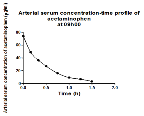
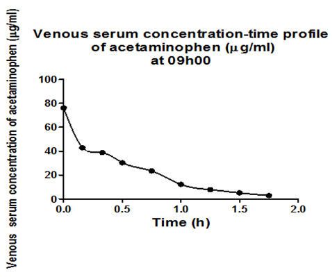
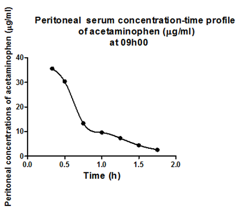
Results obtained after the intramuscular administration of 40mg/kg of acetaminophen to adult male to rats Sprague-Dawley at 09h00 and 21h1 were arbitrarily chosen, to show examples of the results obtained. Figure 1a shows arterial serum concentration-time profile of acetaminophen at 09h00 and description of the observed profile with the developed model of the pharmacokinetic behavior of acetaminophen in adult male Sprague-Dawley rats. Figure 1b shows venous serum concentration-time profile of acetaminophen at 09h00 and description of the observed profile with the developed model of the pharmacokinetic behavior of acetaminophen in adult male Sprague-Dawley rats. Figure 1c shows peritoneal serum concentration-time profile of acetaminophen at 09h00 and description of the observed profile with the developed model of the pharmacokinetic behavior of acetaminophen in adult male Sprague-Dawley rats.1

Figure 1a Observed arterial serum concentration time profile of acetaminophen and the description of the observed profile with the developed model of the dynamic system describing the pharmacokinetic behavior of acetaminophen in adult male Sprague-Dawley rats.

Figure 1b Observed venous serum concentration time profile of acetaminophen and the description of the observed profile with the developed model of the dynamic system describing the pharmacokinetic behavior of acetaminophen in adult male Sprague-Dawley rats.

Figure 1c Observed peritoneal serum concentration time profile of acetaminophen and the description of the observed profile with the developed model of the dynamic system describing the pharmacokinetic behavior of acetaminophen in adult male Sprague-Dawley rats.

The pharmacokinetic dynamic systems used in the current study were mathematical objects, without any physiological significance. They were used to mathematically describe static and dynamic properties of the pharmacokinetic behavior of acetaminophen^18–20 in the male Sprague-Daley rats investigated in the previous study by Bélander et al.¹ The modeling method used in the current study has been described in detail in the studies published previously,^7–16 authored or co authored by the author of the current study. Therefore a description of the modeling method used was not given here.

Analogously as in the previous studies, the development of mathematical models of each dynamic system under study was based on the known input and output of the dynamic system. In general, if dynamic systems are modeled using a transfer function model; as it was the case in the current study (see Eq. (2)), then the accuracy of the models developed depends on the degrees of the polynomials of the transfer function model used to fit the data, see for example the following studies,^7–16 and references therein.

The parameter gain is called also gain coefficient, or gain factor. In general, a parameter gain is defined as a relationship between a magnitude of an output of a dynamic system to a magnitude of an input to a dynamic system in steady state. Or in other words, a parameter gain of a dynamic system is a proportional value that shows a relationship between a magnitude of an output to a magnitude of an input of a dynamic system in the steady state.

The pharmacokinetic meaning of a parameter gain depends on the nature of an investigated dynamic system; see for example full-text articles available free of charge at:

http://www.uef.sav.sk/advanced.htm.

The non-iterative method described in the study published previously²² and used in the current study method allows rapid identification of an optimal structure of a mathematical model of a frequency response function. This is a great advantage of the method used, because it significantly speeds up the process of developing a mathematical model $FM(i\omega j)$   of a frequency response function $FM(i\omega j)$   .

The reason for conversion of $HM(S)$   can be explained as follows: the variable: “ $"S"$  ” in the transfer function model $HM(S)$  in Eq. (2) is a complex Laplace variable, while the variable: angular frequency $"\omega "$  in Eq. (4) is a real variable, what is suitable for modeling purposes.

The current study showed again that mathematical and computational tools from the theory of dynamic systems can be successfully used in mathematical modeling in pharmacokinetics. Frequency response functions are complex functions, therefore modeling is performed in the complex domain. The modeling methods used to develop model frequency response functions are computationally intensive, and for accurate modeling they require at least a partial knowledge of the theory of dynamic system, and an abstract way of thinking about investigated dynamic systems.

The computational and modeling methods that use computational and modeling tools from the theory of dynamic systems can be used for example for adjustment of a drug (or a substance) dosing aimed at achieving and then maintaining required drug (or a substance) concentration–time profile in patients see, for example, the following study.¹⁰

 Moreover, the methods considered here can be used for safe and cost-effective individualization of dosing of a drug or a substance, for example using computer-controlled infusion pumps. This is very important for an administration of a clotting factor to a hemophilia patient, as exemplified in the simulation study.¹⁰

The advantages of the modeling method used in the current study are evident here: The models developed overcome well known limitations of compartmental models: For the development and use of the models considered here, an assumption of well-mixed spaces in the body (in principle unrealistic) is not necessary. The basic structure of the models developed using computational and modeling tools from the theory of dynamic systems, is universal, therefore it is broadly applicable to develop mathematical models not only in the field of pharmacokinetics but also in several other scientific and practical fields. From a point of view of pharmacokinetic community, an advantage of the models developed using computational tools from the theory of dynamic systems is that the models considered here emphasize dynamic aspects¹⁸ of the pharmacokinetic behavior of a drug in a human or an animal body. Transfer functions of dynamic systems are not unknown in pharmacokinetics; see for example the following studies.^26,27 In pharmacokinetics, transfer functions are usually called disposition functions.^28,29

The current study again tried to motivate researchers working in the field of pharmacokinetics to use of an alternative modeling method, namely a modeling method based on the theory of dynamic systems in the development of pharmacokinetic (mathematical) models, as an alternative to traditional pharmacokinetic modeling method.

The mathematical models developed and used in the current study successfully described the pharmacokinetic behavior of acetaminophen after the intramuscular administration to adult male Sprague-Dawley rats ¹. The modeling method used in the current study is universal, comprehensive and flexible and thus it can be applied to a broad range of dynamic systems in the field of pharmacokinetics and in many other scientific or practical fields. The current study again showed that mathematical and computational tools from the theory of dynamic systems can be advantageously used in pharmacokinetic modeling. To see the previous examples illustrating thesuccessful use of the modeling method employed in the current study please visits the author’s website(an English version): http://www.uef.sav.sk/advanced.htm. The current study showed again that an integration of key concepts from pharmacokinetic and bioengineering is a good and efficient way to study dynamic processes in pharmacokinetics, because such integration combines mathematical rigor with biological insight.

About the author

The author is a researcher affiliated with the Institute of Experimental Pharmacology and Toxicology, the Department of Pharmacology of Inflammation Slovak, Academy of Sciences Bratislava, 841 04 Slovak Republic. Her main research interest is to some extant outside her education, because it involves investigations of various dynamic systems in pharmacokinetics, using mathematical models. However, during her work in pharmacokinetics for several years, she successfully utilized her good knowledge of mathematics, based on her engineering education, what is necessary for the development of accurate mathematical models in pharmacokinetics. For more information about the modeling methods used by the author and their use in pharmacokinetic studies, please visit the author’s web page at: www.uef.sav.sk/durisova.htm.

Note

The author worked as a researcher and contractor in the 6FP-Project “Network of Excellence: Biosimulation - A New Tool in Drug Development, contract No. LSHB CT-2004-005137“and in the 7FP-Project “Network of Excellence: Virtual Physiological Human”. Both projects were established by the European Commission. Author worked also in several previous COST program actions. This work of the author in several international projects led to the preparation of the current study.

At present, the author precipitates in the Action BM1204 of the COST program entitled: An integrated European platform for pancreas cancer research: from basic science to clinical and public health interventions for a rare disease, and in Euronanomed II European innovative research & technological development projects in nanomedicine (URL address http://www.euronanomed.net)

The author gratefully acknowledges the financial support obtained from the Slovak Academy of Sciences in Bratislava, Slovak Republic.

None.

None.

1. Belanger PM, Lalande M, Doré F, et al. Time–dependent variations in the organ extraction ratios of acetaminophen in rats. J Pharmacokin Biopharm. 1987;15:133–143.
2. Dedík L, Ďurišová M, Penesová A, et al. Estimation of influence of gastric emptying on shape of glucose concentration–time profile measured in oral glucose tolerance test. Diabetes Res Clin Pract. 2007;77(3):377–384.
3. Iida S, Mizuma T, Sakuma N, et al. Transport of acetaminophen conjugates in isolated rat hepatocytes. Drug Metab Dispos. 1989;17(3):341–344.
4. Brown JM, Udomphorn Y, Suz P, et al. Antipyretic treatment of noninfectious fever in children with severe traumatic brain injury. Childs Nerv Syst. 2008;24(4):477–483.
5. Zurlinden TJ, Reisfeld B.. Physiologically based modeling of pharmacokinetics of acetaminophen and its major metabolites in humans using Bayesian population approach. Eur J Drug Metab Pharmacokinet. 2016;41(3):267–280.
6. van Rossum JM, de Bie JE, van Lingen G, et al. Pharmacokinetics from a dynamical systems point of view. Clin Pharmacokinet Biopharm. 1989;17(3):27–44.  
7. Dedik L, Ďurišová M. Frequency response method in pharmacokinetics. J Pharmacokinet Biopharm. 1994;22(4):237–307.
8. Dedik L, Ďurišová M. CXT–MAIN:A software package for the determination of the analytical form of the pharmacokinetic system weighting function. Comput Methods Programs Biomed. 1996;51(3):183–192.
9. Ďurišová M, Dedík L. Modeling in frequency domain used for assessment of in vivo dissolution profile. Pharm Res. 1997;14(7):860–864.  
10. Ďurišová M, Dedík L. A system–approach method for the adjustment of time–varying continuous drug infusion in individual patients. A simulation study. J Pharmacokinet Pharmacodyn. 2002;29(5–6):427–444.
11. Ďurišová M, Dedík L. New mathematical methods in pharmacokinetic modeling. Basic Clin Pharmacl Toxicol. 2005;96(5):335–342. 
12. Ďurišová M. A physiological view of mean residence times. Gen Physiol Biophys. 2014;33(1):75–80.
13. Ďurišová M. Mathematical model of pharmacokinetic behavior of orally administered prednisolone in healthy volunteers. J Pharmaceut Pharmacol. 2014;2(2):1–5.
14. Ďurišová M. Further worked out examples that illustrated the successful use of an advanced mathematical modeling method based on the theory of dynamic systems in pharmacokinetics. International Journal of Recent Scientific Research. 2015;6(6):4873–4879.
15. Ďurišová M, Dedík L, Kristová V, et al. Mathematical model indicates nonlinearity of noradrenaline effect on rat renal artery. Physiol Res. 2008;57(5):785–788.
16. Ďurišová M. Mathematical model of pharmacokinetic behavior of warfarin. Advances in Pharmacology and Clinical Trials. 2016;1(2):1–7.
17. Levitt DG. PK Quest:A general physiologically based pharmacokinetic model. Introduction and application to propranolol. BMC Clin Pharmacol. 2002;2:5.
18. Weiss M, Pang KS. Dynamics of drug distribution. I. Role of the second and third curve moments. J Pharmacokinet Biopharm. 1992;20(3):253–278.
19. Verotta D. Concepts, properties, and applications of linear systems to describe distribution, identify input, and control endogenous substances and drugs in biological systems. Crit Rev Biomed Eng. 1996;24(2–3):73–139.
20. Xiao H, Song H, Yang Q, et al. A prodrug strategy to deliver cisplatin (IV) and paclitaxel in nanomicelles to improve efficacy and tolerance. Biomaterials. 2012;33(27):6507–6519.
21. Beckermann B, Kaliaguine V. The diagonal of the Padé table and the approximation of the Weyl function of second–order difference operators. Constructive Approximation. 1997;13(4):481–510.
22. Levy EC. Complex curve fitting IRE Trans Automat Contr AC. 1959;4:37–43.
23. Lampariello F, Sciandrone M. Use of the minimum–norm search direction in a nonmonotone version of the Gauss–Newton method. Journal of Optimization Theory and Applications. 2003;119(1):65–82.
24. Boyle P. Options:A Monte–Carlo approach. Journal of Financial Economics. 1977;4(3):323–338.
25. Akaike H. A new look at the statistical model identification. IEEE Trans Automat Contr. 1974;19:716–723.
26. Siegel RA. Pharmacokinetic transfer functions and generalized clearances. J Pharmacokin Biopharm. 1986;14(5):511–552.
27. Segre G. The sojourn time and its prospective use in pharmacology. J Pharmacokin Biopharm. 1988;16(6):657–666.
28. Yates JW. Structural identifiability of physiologically based pharmacokinetic models. J Pharmacokinet Pharmacodyn. 2006;33(4):421–439.
29. Rescigno A. Compartmental analysis and its manifold applications to pharmacokinetics. AAPS J. 2010;12(1):61–72.
30. Gillespie WR, Pedersen VP, Berg MJ, et al. Linear systems approach to the analysis of an induced drug removal process. Phenobarbital removal by oral activated charcoal. J Pharmacokin Biopharm. 1986;14(1):19–28.