In this paper, we present a salient object detection algorithm that based on boundary prior and center prior. First, according to the principle of boundary prior, we construct the Boundary–based map by means of colour distinction. Second, we used colour and location cues to receive the Centre–based map, which based on center prior hypothesis. Then, we exploit the Centre–Bayes map within the Bayesian framework. Finally, we integrated Boundary–based map and Centre–Bayes map into the final saliency map that combined with each features and advantages. Comparing with sixteen methods, experimental results on seven datasets show that our proposed algorithm achieves favourable results in terms of the precision and recall, f–measure and MAE.

Keywords: saliency map; boundary prior; center prior

Recently, as the important field of computer vision, image processing has received considerable attention. In addition, Abundant efforts have been made to find a favourably way to express the content of the image by extracting useful information from image. In this context, the research of salient detection comes into being, the model of saliency is used to find the highlight object in image, and then, it is convenient for the subsequent operations in image processing. Saliency detection can be applied to many modern computer vision tasks, for instance, image classification,¹ image compression,² object location,³ image segmentation.⁴ In the matter of information processing methods, saliency detection algorithms can be divided into top–down and bottom–up methods. The detection algorithm of top–down approaches^5–8 always related to a particular task or target. Before the top–down algorithms find the highlight objects, these algorithms need to obtain the basic properties of target. In this case, the top–down algorithms can quickly and effectively find the salient target in image. But, these kinds of algorithms need to take the supervised learning. On the contrary, the approaches of bottom–up^4,9–12 adopt the low–level visual information without the cues of a certain target. Compared with top–down algorithms, the bottom–up approaches would be more applicable. One of the mostly used bottom–up methods, which measure the distinction between a pixel and region with its neighbourhoods.¹³ Owing to lack of the prior knowledge of the object size, the approach of centre–boundary contrast often calculates the saliency in the multi–scale space; it may increase the computation complexity in some extent. In addition, some researcher adopts the boundary priority,¹² they consider the boundary of image would be more likely to become the background. It is undeniable that the boundary has the high probability being the background, but not all the region in the boundary would be background. Once the salient object locates at the boundary of the image, it may lead to a poor result.

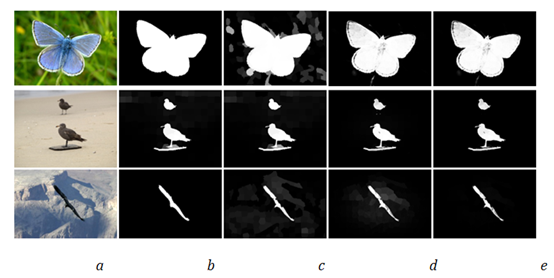
In this paper, we proposed an effective algorithm to solve these problems. For example (Figure 1). Firstly, we consider only one side of the boundary may be the background, and compute the contrast by using the global colour distinction, so we receive a primary saliency map called Boundary–based map, this map can comprehensively find the salient target, but the contrast between the foreground and background may not be significant. So we continue to construct the Centre–based map, this map is based on the center prior assumption.¹⁴ Later the Centre–Bayes map was received by putting the Centre–based map into the Bayesian framework.^15,16 Since the Centre–based map favourably makes up the weakness of the Boundary–based map, we decide to integrate the Boundary–based map and the Centre–Bayes map into the final saliency map.

Figure 1 Saliency maps generated by the proposed algorithm. Brighter pixels reveal higher saliency values.

a. Input image b. Ground truth, c. Bound-based map, d. Centre-Bayes map, e. Saliency map

Recently, the number of algorithms in favour of considering the boundary of image as the background has increased. In Wei et al.¹⁷ construct a feature matrix by contrasting with the boundary, and receive the final saliency map. Qin et al.¹³ Construct a global colour distinction toward boundary seeds, then the saliency map obtained by the iteration of cellular automata. In Yang et al.¹⁸ calculate the relevance between the boundary and whole area of image, and regard the relevance as the saliency for each region. In Wang et al.¹² consider the boundary connectivity as the standard to evaluate the saliency. In addition, some efficient algorithms choose to take the assumption of center prior. Tong et al.¹⁹ exploit a weak map that based on the center prior, and labelled the weak map as the training sample for the strong models. In Chen et al.²⁰ find the salient object with the help of the soft abstraction. In addition, some researcher devotes to the Bayesian framework. In Rahtu et al.⁴ utilize the theory of Bayes to optimize the saliency map. In Xie et al.^15,16 compute the prior probability and likelihood probability of the map; receive the probability of the map by using the Bayes formula. Since those algorithms reveal different effects in detection, and each one has its unique advantages, while we decide to absorb their strengths. Consequently, we proposed our algorithm that based on boundary prior and center prior, and obtained a satisfying result.

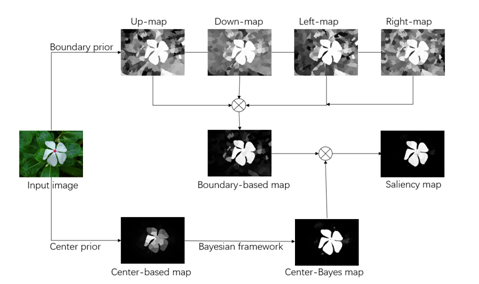
The detailed steps of our salient object detection algorithm showed in Figure 2. At beginning, we consider only one side of image as background. On this account, we construct four global colour distinction maps. Then we integrate them into the Boundary–based map. Using colour and position cues, the Centre–based map exploited by adopting the center prior assumption. After that, we generated the Centre–Bayes map by putting the Centre–based map into the Bayesian framework that based on convex hull. Finally, we construct the final saliency map by integrating the Boundary–based map and the Centre–Bayes map.

Figure 2 The process of our algorithm.

Image features

In order to receive the structure information of image preferably and well preserved salient object boundary. We decide to take the simple linear iterative clustering (SLIC)²¹ algorithm to separate the original image into N small super pixels. SLIC also improves the efficiency of the whole algorithm favourably. Then, we describe the each super pixel rely on the mean colour features and mean coordinates of pixels. We adopt three features, which contained RGB, LAB and Location¹² to represent each super pixel. The experimental results prove that both of the colour features act complementary role in the salient object detection. Also, the Location features can properly compensate the weakness of colour feature in some cases, thus the results of algorithm will be more effective in complex scenes.

Boundary prior

Generally speaking, many algorithms consider the assumption that image boundary will be the background,^12,13,17,18 while some salient object may lie in the boundary of image, therefore, it will impact the quality of saliency map to some extent. To minimize this influence, we consider one side of image boundary as the background. Based on this consideration, we construct four boundary prior maps by the colour distinction. The element ${\text{B}}_t\left(i\right)$ stand for the saliency value of super pixel i in t–th side of image boundary in CIELAB colour space and is calculated as follow

${\text{B}}_t\left(i\right)=\frac{1}{N_t}{\displaystyle \sum }_{j=1}^{N_t}\frac{1}{e^{-\frac{\left|\right|c_i,c_j\left|\right|}{2a^2}}+b}$ (1)

Where $\left|\right|c_i,c_j\left|\right|$  is the Euclidean Distance between the superpixel i and j in the colour space of CIELAB, and $N_t$ (t =1, 2, 3, 4) is the number of super pixels that belonging to each side of image boundary. a, b Is the balance weight. As is showed in the Figure 2, we can intuitively see four boundary prior maps that based on different edge of image. However, these maps are not perfect, but it really reduces the impact of the assumption that the entire image boundary is background. In addition, each prior map has its own advantages, in other words, each of them have some high accuracy areas. Consequently, we integrate this four boundary prior maps into the Boundary–based map:

$B\left(i\right)=B_1\left(i\right)\times B_2\left(i\right)\times B_3\left(i\right)\times B_4\left(i\right)$ (2)

Center prior

The center prior also is considered as an important role in recent detection algorithms [19, 20]. Based on this consideration, we first exploit a location center prior model $\text{g}\left(i\right)$ , it can make the image center more salient and restrain the boundary saliency. Then we construct three correlation matrices by accepting different colour features and Location for all adjacent super pixels (i,j). Later, we compute their relevance [12] $d_f\left(i,j\right)$ as the Euclidean distance between each super pixel.

$d_f\left(i,j\right)={\displaystyle \sum }_{i,j=1}^{N}d\left(i,j\right)$  (3)

Where N is the number of the super pixels. According to the experiential information, we define that a superpixel has no relevance to itself, so we define $d_f\left(i,j\right)=0$ . Then, we generate the Centre–based map that combined with three correlation matrices $d_f\left(i,j\right)$ and location center prior model $\text{g}\left(i\right)$ . The method was shown as shown below:

$C\left(i\right)=\text{g}\left(i\right)\times {\displaystyle \prod }_{f=1}^3(\frac{1}{N_b}{\displaystyle \sum }_{j=1}^{N_b}{d}_f\left(i,j\right))$  (4)

 The $f$  represent different feature spaces, $f=1$ represent the RGB, $f=2$ represent the CIE Lab, and $f=3$ represent the Location feature. $N_b$ is the number of the boundary super pixels. There is a point here, we must normalized $d_f\left(i,j\right)$  and $\text{g}\left(i\right)$ into [0, 1]. Predictably, Centre–based map has the characteristic that the super pixel which closer to the center of image has a higher weight. In spite of the most of the object will locate at the center of image, but this assumption will easily influence the prior map by the object distribution. To reduce the impact, we decide to put the Centre–based map into the Bayesian framework. In Bayesian framework, we calculate the likelihood probability with the help of the convex hull,15,16 For one hand, the framework makes up the insufficient of center prior model, on the other hand, it really strengthens the saliency of object further. A Centre–Bayes map that entirely different with the Boundary–based map has constructed.

Integration

Now, we already generated two saliency maps roughly. Boundary–based map and Centre–Bayes map have complementary properties. The Boundary–based map not only works well in revealing the global colour distinction, but also perfectly preserves the whole information of the salient object. However, the Boundary–based map may have the low contrast ratio for the foreground and background, thus it will reduce the accuracy of the algorithm. On the contrary, the Centre–Bayes map favorably highlighted the saliency regions, but sometimes the saliency map would be affected by the object distribution and cannot emphasize object completely. According to this situation, we make full use of advantages of each saliency map and integrate them into the final saliency map:

$M={\displaystyle \sum }_{i=1}^N\left(\text{B}\left(i\right)\times \text{C}\left(i\right)\right)$  (5)

Where $N$ is the number of the super pixels. $\text{B}\left(i\right)$  is the Boundary–based map and $\text{C}\left(i\right)$ is the Centre–Bayes map. $M$  is the final saliency map in our algorithm.

We evaluate the algorithms based on seven widely used datasets in saliency detection filed. They are ASD,²² MSRA–5000,²³ THUS,²⁴ ECSSD,¹¹ THUR,²⁵ PASCAL²⁶ and SED2.²⁷ ASD contains 1000 images, and most images are relatively simple. MSRA5000 contains 5000 images with accurate masks. THUS contains 10000 images, labelled with pixel–wise ground truth masks. ECSSD contains 1000 semantically meaningful but structurally complex images. THUR contains 6232 images, which have complex backgrounds. PASCAL contains 1500 images with complex scenes. SED2 contains 100 images with two targets. We compare our algorithms with the comparatively advanced or classic algorithms. They are IT98,²⁸ FT09,²² CA10,²⁹ RC11,³⁰ SVO11,³¹ XL11,¹⁵ GS12,¹⁷ SF12,³² XL13,¹⁶ PCA13,³³ HS13,¹¹ LMLC13,²⁰ GC13,¹⁷ GMR13,¹⁸ wCO14,¹² LPS15.³⁴

Evaluation metrics

In this paper, we take the standard precision–recall curves to evaluate all algorithms, which we decide to compare with. We draw P–R curves by using threshold value segmentation. First, we normalized the saliency map, which we evaluate into the range [0,255], then set a threshold every 5 value, and we receive a series of binary map. We contrast with the ground–truth to compute the precision and regression rate, and draw the P–R curves. An efficient algorithm not only required high precision but also a high recall value, thus we consider F–measure as the comprehensive evaluate principle:

$F_{\phi }=\frac{\left(1+{\phi }^2\right)•precision•recall}{{\phi }^2•precision+recall}$ (6)

Where, according the previous paper [13], we set the ${\phi }^2$ to 0.3 to show the relative importance. In addition, we compute the value of mean absolute error (MAE) [22], it similar to P–R curves, MAE calculates the average distinction between the saliency map and ground–truth:

$MAE=\frac{1}{H}{\displaystyle \sum }_{h=1}^H\left|S\left(h\right)-GT\left(h\right)\right|$ (7)

The evaluate method mainly used in the area of image segmentation, and it reveal the similarity between the salient map and ground–truth.

Validation of the proposed algorithm

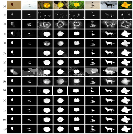
To show the effectiveness of our method, we test our algorithm in seven datasets. P–R curves and F–measure histograms in Figure 3 and MAE values in Table 1 reveal that: 1, our method generate a favourably result. 2, our method can adapt different image background. Figure 4 is the comparison of saliency maps on different datasets.

Figure 3 Comparative maps on seven datasets.

Figure 4 Comparison of saliency maps on different datasets.

 (a) input images (b) IT (c) CA (d)RC (e) SF (f) HS (g) GMR (h) LMLC (i) PCA (j) GC (k) wCO (l) LPS (m) Ours (n) GT

In this paper, we proposed a bottom–top method to exploit a saliency map based on the prior principle of boundary and centre. Based on the assumption, we consider the difference and similarities between the boundary and background, thus we can exploit the Boundary–based map. Meanwhile, because of center prior, we construct the Centre–based map that has high precision, then we take it into the Bayesian framework to achieve a further improved map called Centre–Bayes map. Our algorithm benefits their advantages, and improves their weakness by integrating them into the final saliency map, which has higher precision and recall. Experimental proved that our algorithm could receive a favourable result in different datasets.

The research was supported by the National Science Foundation of China (No. 61502220, No. U1304616 and No. 61472245).

Author declares that there are none of the conflicts.

References

- Siagian C, Itti. Rapid Biologically–Inspired Scene Classification Using Features Shared with Visual Attention. IEEE Trans Pattern Anal Mach Intell. 2007;29(2):300–312.
- Itti L. Automatic foveation for video compression using a neurobiological model of visual attention. IEEE Trans Image Process. 2004;13(10):1304–1318.
- Gao D, Han S, Vasconcelos N. Discriminant saliency, the detection of suspicious coincidences, and applications to visual recognition. IEEE Transactions on Pattern Analysis & Machine Intelligence. 2009;31(6):989–1005.
- Rahtu E, Kannala J, Salo M, Janne Heikkilä. Segmenting Salient Objects from Images and Videos. Computer Vision–ECCV. 2010. p. 366–379.
- Alexe B, Deselaers T, Ferrari V. What is an object? IEEE Conference on IEEE. 2010. p. 73–80.
- Jiang H, Wang J, Yuan Z, et al. Salient Object Detection: A Discriminative Regional Feature Integration Approach. IEEE Computer Society. 2013. p. 2083–2090.
- Ng AY, Jordan MI, Weiss Y. On Spectral Clustering: Analysis and an algorithm. Proceedings of Advances in Neural Information Processing Systems. 2002. p. 849–856.
- Yang J. Top–down visual saliency via joint CRF and dictionary learning. IEEE Trans Pattern Anal Mach Intell. 2017;39(3):576–588.
- Hou X, Zhang L. Saliency Detection: A Spectral Residual Approach. IEEE Conference on Computer Vision and Pattern Recognition. 2007. 1–8.
- Klein DA, Frintrop S. Center–surround divergence of feature statistics for salient object detection. IEEE Computer Society. 2011;50(2):2214–2219.
- Yan Q, Xu L, Shi J, et al. Hierarchical saliency detection. IEEE Conference. 2013. p. 1155–1162.
- Zhu W, Liang S, Wei Y, et al. Saliency Optimization from Robust Background Detection. IEEE Conference on Computer Vision and Pattern Recognition. 2014. p. 2814–2821.
- Qin Y, Lu H, Xu Y, et al. Saliency Detection via Cellular Automata. IEEE Conference. 2015. p. 110–119.
- Liu T, Yuan Z, Sun J, et al. Learning to detect a salient object. IEEE Transactions on Pattern Analysis & Machine Intelligence. 2011;33(2):353–367.
- Xie Y, Lu H. Visual Saliency Detection Based on Bayesian Model. IEEE International Conference on Image Processing. 2011;263(4):645–648.
- Xie Y, Lu H, Yang MH. Bayesian saliency via low and mid level cues. IEEE Trans Image Process. 2013;22(5):1689–1698.
- Wei Y, Wen F, Zhu W, et al. Geodesic Saliency Using Background Priors. European Conference on Computer Vision. 2012. p. 29–42.
- Yang C, Zhang L, Lu H, et al. Saliency Detection via Graph–Based Manifold Ranking. IEEE Conference on Computer Vision and Pattern Recognition. 2013. p. 3166–3173.
- Tong N, Lu H, Xiang R, et al. Salient object detection via bootstrap learning. IEEE Conference on Computer Vision and Pattern Recognition. 2015. p. 1884–1892.
- Cheng MM, Warrell J, Lin WY, et al. Efficient Salient Region Detection with Soft Image Abstraction. IEEE ICCV. 2013. p. 1529–1536.
- Achanta R, Shaji A, Smith K, et al. Slic super pixels. EPFL Technical report. 2010. p. 1–15.
- Achanta R, Hemami S, Estrada F, et al. Frequency–tuned salient region detection. IEEE International Conference on Computer Vision and Pattern Recognition. 2009. p. 1597–1604.
- Cheng MM, Mitra NJ, Huang X. Salient Object Detection and Segmentation. IEEE Transactions on Pattern Analysis & Machine Intelligence. 2011;37(3):1–14.
- Cheng MM, Mitra NJ, Huang X, et al. Salient Shape: group saliency in image collections. Visual Computer International Journal of Computer Graphics. 2014;30(4):443–453.
- Everingham M, Gool LV, Williams CKI, et al. The Pascal, Visual Object Classes (VOC) Challenge. International Journal of Computer Vision. 2010;88(2):303–338.
- Alpert S, Galun M, Basri R, et al. Image Segmentation by Probabilistic Bottom–Up Aggregation and Cue Integration. IEEE Transactions on Pattern Analysis & Machine Intelligence. 2007;34(2):1–8.
- Itti L, Koch C, Niebur E. A Model of Saliency–Based Visual Attention for Rapid Scene Analysis. IEEE Transactions on Pattern Analysis & Machine Intelligence. 1998;20(11):1254–1259.
- Goferman S, Zelnik–Manor L, Tal A. Context–aware saliency detection. IEEE Trans Pattern Anal Mach Intell. 2012;34(10):1915–1926.
- Cheng M, Zhang G, Mitra NJ, et al. Global contrast based salient region detection. IEEE Conference. 2011;37(3):569–582.
- Chang KY, Liu TL, Chen HT, et al. Fusing generic object ness and visual saliency for salient object detection. IEEE International Conference on Computer Vision. 2011. p. 914–921.
- Hornung A, Pritch Y, Krahenbuhl P. Saliency filters: Contrast based filtering for salient region detection. IEEE Conference on Computer Vision and Pattern Recognition. 2012. p. 733–740.
- Margolin R, Tal A, Zelnik–Manor L. What makes a patch distinct? Computer Vision and Pattern Recognition (CVPR). 2013. p. 1139–1146.
- Li H, Lu H, Lin Z, et al. Inner and inter label propagation: salient object detection in the wild. IEEE Transaction on Image Processing. 2015. p. 3176–3186.
©2017 Jiang, et al. This is an open access article distributed under the terms of the,
which
permits unrestricted use, distribution, and build upon your work non-commercially.