Analysis for angular velocity of railway wheelset measurement and creep error estimation

doi:10.15406/iratj.2019.05.00175

eISSN: 2574-8092

International Robotics & Automation Journal

Research Article Volume 5 Issue 2

Analysis for angular velocity of railway wheelset measurement and creep error estimation

Zulfiqar Ali Soomro

Verify Captcha

Regret for the inconvenience: we are taking measures to prevent fraudulent form submissions by extractors and page crawlers. Please type the correct Captcha word to see email ID.

Mechanical Engineering Department, Quaid-e-Awam University of Engineering Science and Technology, Pakistan

Correspondence: Zulfiqar Ali Soomro, Mechanical Engineering Department, Quaid-e-Awam University of Engineering Science and Technology Nawabshah (Sind), Pakistan

Received: February 14, 2019 | Published: April 3, 2019

Citation: Soomro ZA. Analysis for angular velocity of railway wheelset measurement and creep error estimation. Int Rob Auto J. 2019;5(2):63-67. DOI: 10.15406/iratj.2019.05.00175

Download PDF

Abstract

The rotational speed of the railway wheelset connected by solid axle is crucial problem for proper running of vehicle due to unbalanced ratio of adhesion and creep level owing to contaminated conditions to cause fatal damage. In this paper, the angular velocity of rail road wheels is modeled by its concerned dynamics. This dynamics is altered to kalman filter folded by relative formulations to estimate the noise caused through measurements by actual signals. Thus error percentage is determined by these two wheels separately to detect the adhesion based upon creep coefficient to control slippage of wheelset.

Keywords: solid axle, adhesion, creep co-efficient, kalman filter, covariance, noise, slip

Introduction

The dynamic analysis concerned to the vertical railroad wheel contact usually rises on increase of railway train velocity. In scarce conditions, the relevant distance of railway wheels excitants by the broadly band and discrete disturbances available on the moving contacts of wheelset and railroad can tend to extra contacting forces. In the work done by,¹ the influence of railway wheelset rotation was conceived by modeling rail-wheel implied to a rotating force surrounding its perimeter at constant angular speed. Thus inertial forces are ignored. The procedure provided by² is used to set up the motion equations for the rotating of rail wheelset. This paves path for structuring to small elastic deformations for huge translations and rotations concerned railway dynamics.

It can be conceived that there is angular speed as contacting point between the rail profiles and wheelset. By watching the wheel profile, this point discriminates the undulating radii of wheels. In the central position, the rolling radii for the left and right wheels are equal due to the symmetry of the rail wheelset system.³ A lateral distance due to the wheelset motion creates dissimilarity between the rolling radii of wheels running on a straight track ends in a timely motion of the railway wheelset, as stated theoretically by Klingel known as the Klingel movement of wheels.

A more dependable method of checking the dynamics of railway vehicles comprises of examining the actual vehicles circulating attitude on the railway track.⁴ The railway vehicle wheels and track are correlated in the rail-wheel contact zone. Here, almost the forces that assure the stability of vehicle along with the railroad track are applied.^5,6 In such situation, no any transversal forces are implied on the railway wheels with a perfect symmetry between the left and right wheels and railroad profiles.

The hybrid re-adhesion methods based on the relative velocity measurement are described.^7,8 These controllers having precise measurement of the railway vehicle and wheelset rotational velocities make it complicated to get the preferable efficiency. Another methodology concerned to disturbance estimators are proposed to detect the slipping conditions for trains.^9,10

Kalman filter is a beneficial tool to filter the parameters of a linear stochastic process for the railway wheelset with required track disturbance, by known processing outputs and the model parameters. The system has linearized the nonlinear creepages at specific point on the creeping curves. This research uses a newer technique to recognize the rail-wheel contacting conditions by checking the alterations in the dynamic virtues of the rail wheelset as the vehicle travels through the rail track. The proposed scheme indirectly uses the contacting conditions with minimal measure requiring system. The results described show the satisfactory performing efficiency.¹¹

In this paper, the angular velocity of rail wheelset is discussed in second section and kalman filter is designed in third section while in 4^th section simulation results are presented.

Wheelset dynamics

In following Figure 1, Railway wheelset contains of two left and right wheels joined rigidly by solid axle in such a way that the two wheels rotate with some velocity. The wheelset are joined to bogie through suspension parts of railway train. The purpose of the suspension parts is to apart the passenger car from the vertical distance produced by disturbances in railroad. Along with riding comfort, the suspension works to ameliorate the stability of the railway wheels.¹²

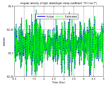
Figure 1 Right wheel co-efficient of creep at 10⁷.

The railway wheelset having two wheels rigidly fastened by axle are the frustums of a cone with sloping roll on rail surfaces being an arc of a circle with radius. This restoring force from the flanges on the wheels is fixed by a bold linearly spring with a dead band and no any damping factor with bogies.¹³

When wheelset is dislocated sideways then creep for both sides wheel is shown as under, where longitudinal creep ‘λ’ is correlated with wheel velocities.¹⁴

$λ_{x} = \frac{V_{w} - V}{V}$ (1)

Here V_w is linear velocity as

$V_{w} = W_{w} . r_{o}$ (2)

$v_{w} = w_{w L} + w_{w R}$ (3)

The left and right wheel speeds are as under

$v_{w L} = ω_{w L} . [r_{o} + γ (y - y_{t})]$ (4)

$v_{w R} = ω_{w R} . [r_{o} - γ (y - y_{t})]$ (5)

Here $y_{t}$ =noise, $γ$ = conicity $F_{x R} = f_{11} λ_{x R}$ (6) and $F_{x L} = f_{11} λ_{x L}$ (7) here F_X =creep forces and f₁₁ = creep coefficient.

Kalman filter design

The Kalman filter is used for estimation of linearly systems and the extended Kalman filter is used for nonlinearly stochastic systems for estimation of dynamic systems.¹⁵ Usually kalman filter uses as an observer for fault detection during disturbances. The Kalman estimator is one of the most famous methods applied for states and parameter estimation during noise. It uses concerned measurements that are correlated linearly to the state and error covariance matrices to create a gain concerned to Kalman Gain in its phenomenon. This gain is used to the prior state estimation producing a posterior estimation. The estimation process occurs in a predictor-corrector way by maintaining a statistically minimal state error covariance matrix in kalman filter analysis. Equation (8) is practical to design the Kalman filter in this paper. Basic linear rail wheelset equations based on linearly creeping forces relationships in equations (1) to (7) on straight railroad with tracking input noise y_t are given below in state variable form.

$ω_{R} = - \frac{r_{o}^{2} f_{11}}{v I_{R}} - \frac{γ f_{11}}{I_{R}} y_{t}$ (8)

$ω_{L} = - \frac{r_{o}^{2} f_{11}}{v I_{L}} ω_{L} + \frac{γ f_{11}}{I_{L}} y_{t}$ (9)

$[\begin{array}{l} w_{R} (n + 1) \\ w_{L} (n + 1) \end{array}] = [\begin{matrix} - \frac{r_{o}^{2} f_{11}}{v I_{R}} & 0 \\ 0 & - \frac{r_{o}^{2} f_{11}}{v I_{L}} \end{matrix}] [\begin{array}{l} w_{R} (n) \\ w_{L} (n) \end{array}] + [\begin{array}{l} - \frac{γ f_{11}}{I_{R}} \\ \frac{γ f_{11}}{I_{L}} \end{array}] y_{t}$ (10)

Where, n = 0, 1, 2, ... ;

The errors of this estimating model, and inducted errors of yaw pace and other dynamic terms are considered as the process noise. This noise is given by y_t as denoted in equation (4, 5). This caused disturbance is filtered by kalman filter.^16,17

$w_{n} = [\begin{array}{l} w_{R} (n) \\ w_{L} (n) \end{array}]$ (11)

The equation of measurement is as under $y (n) = (\begin{matrix} 1 & 0) [\begin{array}{l} w_{R} (n) \\ w_{L} (n) \end{array}] + y_{t} \end{matrix}$ (12)

In equation (12), y_t is the noise measurement. Hence state space model is used to estimate angular velocity is given by

$X_{n + 1} = Φ X_{n} + W_{n}$ (13)

$y_{n} = H X_{n} + V_{n}$ (14)

Where, $X_{n} = [\begin{array}{l} w_{R} (n) \\ w_{L} (n) \end{array}]$ $X_{n + 1} = [\begin{array}{l} w_{R} (n + 1) \\ w_{L} (n + 1) \end{array}]$ , and $Φ = [\begin{matrix} - \frac{r_{o}^{2} f_{11}}{v I_{R}} & 0 \\ 0 & - \frac{r_{o}^{2} f_{11}}{v I_{L}} \end{matrix}]$ are state vectors at steps n and n+1 and H=[l 0] is the matrix of wheel speed measurement. Wn and y_t are used as white noise of zero average, so the noise covariance is assumed as $Q = [\begin{matrix} 0.001 & 0 \\ 0 & 0.01 \end{matrix}]$ The noise covariance R and its determination of is the longitudinal speed estimated technique based on kalman filter.^18‒20 The steady-state Kalman filter gain K, is calculated by applying the equations (10) and (11), therefore the relevant equation of Kalman filter is agreed by

$X_{n + 1} = [Φ - K_{f} H] X_{n} + K_{f} y_{n}$ (14)

Simulation results

The angular velocity of wheelset is replicated to determine three different creep co-efficient attitudes. The Kalman filter techniques are applied to estimate actual parameters by their measurements as described as under.

Right wheel angular velocity of at various co-efficient of creep

The right wheel angular velocity of the wheelset is shown in above Figure 1. Whereas right wheel angular velocity is checked by creep co-efficient at 10⁷ to stare at the recital of the right side wheel.^17,18

In Figure 1, the initial angular velocity of right wheel 92.38 rad/sec varies to 92.48 rad/sec with stepped rate of 0.04 rad/s with respect to time laps from 0.5 sec to 5 sec with increase of 0.5 seconds. The actual signal is shown by ‘blue colour’ rides with the estimated signals displayed by ‘green colour’ in bedlam way denote commotion in main waives and trim in middle.

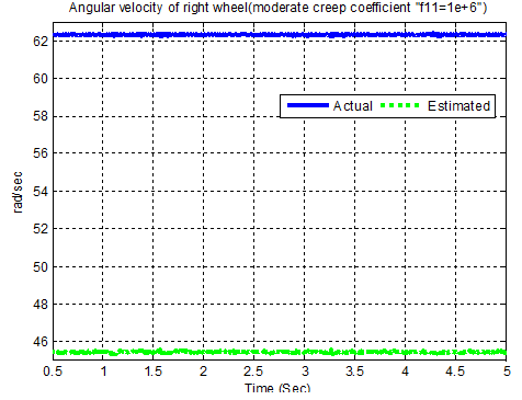
The Figure 2 shows that right wheel angular speed alters from 45.5 rad/sec as estimated limitation and 62.3 rad/s for the actual sign with flooring in time 0.5 sec to 5 seconds when creep co-efficient is planned as 10⁶.^.The estimated and actual standards change apart from each other. This means both curves become apart from each other on reducing the co-efficient of creep charge.

Figure 2 Right wheel creep co-efficient of 10⁶.

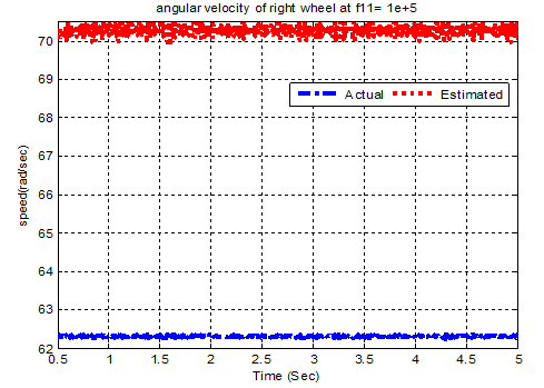
In Figure 3, On assuming the creep co-efficient as 10⁵ then right wheel angular velocity changes from somewhat closer to 70.5 rad/sec as for the estimated restriction and earlier to 62.2 rad/sec for the actual indication with flooring within time 0.5 sec to 5 sec. The estimated and actual signals are at distant from each other. The creep coefficient values vary according to the material properties and environment conditions.

Figure 3 Right wheel creep co-efficient of 10⁵.

The results obtained from both Figure 2 and Figure 4, vary inversely with each except the image of the Figure 1, reflects that when the co-efficient of creep is superior then estimated and actual signals partly cover each other, and estimated and actual signals are detached from each other when creep co-efficient is decreased. Whereas in Figure 3 both estimated curve and actual parameter travel also a partly but differently to as in Figure 2.

Left wheel angular velocity of at various co-efficient of creep

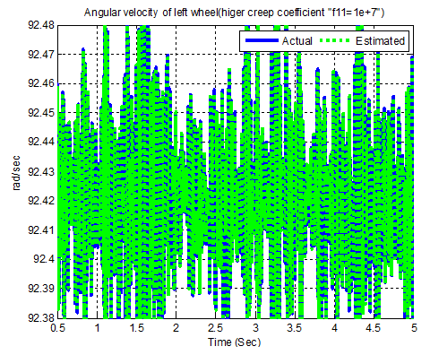
The left wheel angular velocity of wheelset is displayed in the Figure 4 to Figure 6, where left wheel angular velocity is checked by three diverse creep co-efficient to observe its performance. The creep coefficient is the variable parameter, which depends upon the ratio and level of adhesion applications affected by contamination.¹⁷

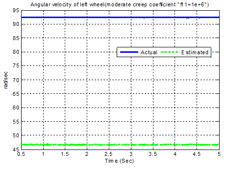
Figure 4 Left wheel creep co-efficient of 10⁷.

Figure 5 Left wheel creep co-efficient at 10⁶.

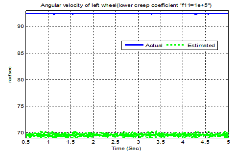
Figure 6 Left wheel creep co-efficient at10⁵.

In Figure 4, when co-efficient of the creep is taken at 10⁷for left wheel. We observe that left wheel moves with its angular velocity of 92.38 rad/sec to 92.48 rad/sec for estimated curve denoted by ‘red colour’ within time limits 0.5 sec to 5 sec with augmentation of 0.5 sec. While actual signal denoted by ‘blue colour’ travels with estimated signals in anarchy way viewing certain riot in big waive and thin in the centre with identical time. The Figure 5, left wheel angular velocity for estimated signal runs on 46.5 rad/sec by creep co-efficient value of 10⁶and 93.2 rad/sec for the actual signal with time from 0.5 sec to 5 sec. These both values differ by more distant from one other.

In Figure 6, left wheel angular velocity for estimated signal runs on varies from 69 rad/sec slightly below 70 rad/sec by creep co-efficient value of 10⁵ and 94.5 rad/sec for the actual signal with time variation of 0.5 sec to 5 sec. both estimated and actual signals also contrast and run at so much away from each other.

Error estimation for angular speeds

Below is representation of right and left rail wheels

Estimation of error for angular speed of right wheel

The error is estimated for angular speed of right wheel through blue line and green line for elevated (10⁷) and subordinate (10⁵) coefficient of creep.

The error estimation ratio for right wheel based upon higher and lower coefficient of creep is denoted in Figure 8. The higher co-efficient of creep displayed in ‘blue line’ runs on straight path of zero error scale. This conceives that there is maximum adhesion to resist slip. While lower co-efficient of creep displayed in ‘green line’ ranging from 13 to 23 on vertical scale zigzag pattern to end at 17.3 of error % in slim means that adhesion is imperfect.

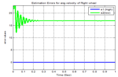
Figure 7 Error estimation for right-wheel speed.

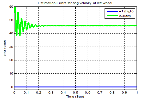
Figure 8 Error estimation for left wheel speed.

The Figure 7 shows ‘e1’ as error estimation for higher coefficient of creep and ‘e2’ as for error estimation for higher coefficient of creep depending upon their sizes.

Estimation of error for angular speed of left wheel

The error estimation for angular speed for left wheel is classified by higher coefficient of creep as 10⁷through blue line and green line for lower coefficient of creep as 10⁵. The Figure-8 shows error estimation by ‘e1’ for higher creep coefficient and ‘e2’ error estimation for lower coefficient of the creep. Whereas when moderate error is encountered then that will show marginal irregularity.^17,18

The quoted high and low coefficient of creep sizes are used to guess the error ratio for left wheel of the railway in fig-8 as below. The blue line denotes higher coefficient of creep travels on zero scale vertically. This shows no error in adhesion to face slip. Whereas lower creep coefficient displayed by green line passes through 46 on vertical scale of error denotes the defect of adhesion to cause slip.

Conclusion

In this paper, the dynamics for angular speeds of left and right railway wheelset is modeling is discussed. The kalman filter (KF) is designed by mathematical model through formulations. This kalman filter is used to estimate the noise through measurements by actual parameters. From simulation results, it can be analyzed that the left wheel angular speed is also better than that of the speed of right wheel during estimation by kalman filter through application of different co-efficient of creep. Here both rail wheels signals behave in same nature of direction with different values. Similarly the error value is detected for both railway wheels, where in both wheels slip becomes zero indicating proper ratio of adhesion on higher creep of co-efficient. Whereas both left and right rail road vehicle wheels behave with different values in same nature on lowering creep coefficient ratio. Thus it can be concluded that on enhancing the value of creep coefficient, both estimated and actual parameters for both values run collectively and consequently error ratio becomes zero to avoid chance of slip. While on reducing creep coefficient value the travel separately with noise in error ratio then it is balanced after some span of time.

References

- Thompson DJ. Wheel–rail noise generation. Part V: inclusion of wheel rotation. Journal of Sound & Vibration. 1993;161(3): 467–482.
- Shabana AA. Dynamics of multibody Systems. 3rd ed. USA: Cambridge University Press; 2005.
- Attivissimo Filippo, Angelo Danese, Nicola Giaquinto, et al. (2007) A railway measurement system to evaluate the wheel–rail interaction quality. IEEE Transactions on Instrumentation and Measurement. 2007;56(5):1583‒1589.
- Esveld C. Modern Railway Track. 2nd ed. Netherlands: MRT‒Prod. 2001. 87 p.
- Pepe D. The issues of wheel–rail contact geometry: Measure techniques of the parameters concerned. Proc Int Wheelset Congr. 2001. p. 17–21.
- Binghua Huang, Zhen Fu Chen. Latest trends and development trends of ESC. J Automotive Engineering. 2008;30(1):1‒9.
- Choi H, Hong S. Hybrid Control for Longitudinal Speed and Traction of Vehicles. 28th Annual Conference on IEEE Industrial Society. 2002;2:1675‒1680.
- Park D. Moon‒Sup K, Don‒Ha H, et al. Hybrid Re‒Adhesion Control Method for Traction System of High‒Speed railway. Proceedings of the 5th International Conference on Electrical Machines and Systems. 2001. p. 739‒742.
- Kim W, Kim Y, Kang J, et al. Electro‒Mechanical Re‒Adhesion Control Simulator for Inverter‒Driven Railway Electric Vehicle. Proceedings of the 34th IEEE Industrial Application Conference. 2002;2:1026‒1032.
- Hussain I, Mei TX, Jones AH. Modeling and Estimation of Nonlinear Wheel‒Rail Contact Mechanics. Proceedings of Twentieth International Conference on System Engineering. 2009. p. 219‒223.
- Nath Y, Athre K, Jayadev K. Non Linear Dynamics of Railway Wheel Set. National conference on nonlinear systems & dynamics, NCNSD. 2003. p. 233‒236.
- Mei TX, Yu J, Wilson D. A Mechatronics Approach for Effective Wheel Slip Control in Railway Traction. IFAC Proceedings Volumes. 2008;41(2):8275‒8280.
- Li Ping, Roger Goodalla, Paul Weston, et al. Estimation of railway vehicle suspension parameters for condition monitoring. Control Engineering Practice. 2007;15(1):43‒55.
- Ru J, Li R. Variable‒structure multiple‒model approach to fault detection, identification and estimation. IEEE Trans. Control Syst. Technol. 2008;16(5):1029–1038.
- Mei TX, Li H, Goodall RM. Kalman filters applied to actively controlled railway vehicle suspensions. Transactions of the Institute of Measurement and Control. 2001;23(3):163‒181.
- Soomro ZA. Adhesion detection analysis by modeling rail wheel set dynamics under the assumption of constant creep coefficient. Mechatronics. Electrical Power and Vehicular Technology. 2014;5(2):99‒106.
- Soomro ZA. Development of Onboard adhesion identification system for railway vehicles. 2015.
- Soomro ZA. Computation of Slip analysis to detect adhesion for protection of rail vehicle and derailment. Journal of Applied and Computational Mechanics. 2015;1(3):145‒151.
- Soomro ZA. Detection of lateral motion noise and error ratio for rail wheelset based upon creep. Technical journal. University of Engineering and Technology (UET) Taxila, Pakistan. 2016;21(3):64‒68.
- Soomro ZA. Dual estimation of lateral analysis for railway vehicle wheelset to control disturbance for smooth running. AUSMT. 2017;7(3):1‒5.
©2019 Soomro. This is an open access article distributed under the terms of the,
which
permits unrestricted use, distribution, and build upon your work non-commercially.