Submit manuscript...
International Journal of
eISSN: 2475-5559

Petrochemical Science & Engineering

Research Article Volume 3 Issue 4

Modeling of the thermodynamic properties of the methylamine/water refrigerant mixture

Khalifa Mejbri,1 Ahmed Bellagi2

1National Engineering School, University of Monastir, Tunisia
2National Engineering School, University of Monastir, Tunisia

Correspondence: Khalifa Mejbri, National Engineering School, University of Monastir, Av. Ibn El Jazzar, 5000 Monastir, Tunisia, Tel (+216) 53782393

Received: May 01, 2018 | Published: October 25, 2018

Citation: Mejbri K, Bellagi A. Modeling of the thermodynamic properties of the methylamine/water refrigerant mixture. Int J Petrochem Sci Eng. 2018;3(5):161-170. DOI: 10.15406/ipcse.2018.03.00090

Download PDF

Abstract

This paper presents the prediction of the phase behavior of methylamine/water refrigerant mixture. To do so, two equations of state were investigated: PC-SAFT and GEOS. The adjustable specific parameters of pure fluids are determined by regression of vapor pressure and saturated liquid and vapor density data. The calculations show that the GEOS model predicts more accurately the thermodynamic properties of pure fluids, in particular in the vicinity of the critical point. For binary mixtures, the cross-interaction parameters are obtained by regression of the vapor-liquid equilibrium data available in the literature. The comparison between predicted and experimental data reveals that both investigated EOS have comparable performance with slight superiority to GEOS when approaching the critical temperature of methylamine. Finally, since the GEOS model is more mathematically tractable and more accurate when applied to pure fluids, it is adopted for the correlation and prediction of the thermodynamic properties of the methylamine/water system.

Keywords: methylamine, water, thermodynamic, properties, equations, PC SAFT, GEOS

Introduction

Absorption refrigeration machines represent a promising solution in order to circumvent the increase in electric power consumption due to air-conditioning and refrigeration particularly in the summer period. This technique for the production of cold exhibits some interesting advantages. By using heat as driving energy, such that released by the combustion of natural gas or LPG, it is possible to by-pass the usage of electric power. Moreover, this method allows the valorization of the thermal emissions of intermediate temperatures. The electric power needed is marginal (i.e., essentially for circulation pumps and control systems). However, the absorption cycles are much more complex in comparison to the vapor compression machines. On the energy performance level, the single-effect absorption refrigeration chillers present a COP (between 0.5 and 0.7) lower than its counterpart obtained with the vapor compression systems, even when brought back to the primary energy. Hence, the absorption technique for production of cold is not energy efficient. However, this concern becomes secondary if the supplied driving heat is inexpensive (e.g., heat from thermal discharges or from thermal solar energy plants). Under these circumstances, the absorption refrigeration may well constitute a viable alternative to the vapor compression systems. During last decades, many studies in this field have focused on the standard systems water-ammonia and water-LiBr solutions and theoretical and experimental investigations of other alternative working fluids. This quest was aimed at the development of techniques, which improve absorption systems performance and make them economically competitive when compared to the conventional compression vapor systems.121 The absorption heat transformers are also investigated with interest for waste-heat reutilization within industrial processes, due to their favorable economics and mild environmental effects.2228

The thermal performance of an absorption refrigeration system is greatly dependent on the physical and chemical properties of the working fluids used.29–31 Up to now, only two refrigerant mixtures, NH3-H2O and LiBr- H2O, are widely employed in commercialized absorption chillers. However, these working fluids present some limitations. Firstly, the LiBr- H2O system works at high vacuum levels, which are difficult to maintain. Secondly, this mixture cannot be used for air-cooled units under high ambient air temperatures due to salt crystallization.32–34 Further, with water as refrigerant temperatures lower than 0°C are not possible. On the other hand, the NH3-H2O mixture is such that the boiling temperature difference between the absorbent (water) and refrigerant (ammonia) of is not sufficiently large, which makes necessary a rectification step at the exhaust of the boiler to ensure the required purity of the desorbed ammonia. In addition, the driving heat has to be supplied to the generator at a high temperature of about 180°C. In order to circumvent the limitations of the NH3-H2O system, a large number of studies has focused on the search for alternative and more appropriate fluid mixtures.35–37 The looked-for working fluid system should exhibit the desired properties in particular keep the condenser pressure at the lowest possible level above one bar, allowing low generator temperatures, and hence making the use of low-grade thermal sources as driving heat. A potential candidate is water/methylamine system with methylamine replacing ammonia as refrigerant. It has been found that the thermodynamic properties of the methylamine–H2O mixture are interesting for application in absorption refrigeration.38–40 Vapor pressures and driving temperatures data indicate that thermal energy sources at low temperatures may be used (e.g., solar, geothermal and waste heat of industrial and commercial processes). However, methylamine is a refrigerant that has been poorly investigated in the literature. Indeed, property data for the pure fluid and its solutions with several solvents are scarcely reported in the literature. Some thermodynamic properties of methylamine–H2O mixtures are found in references,41–51 occasionally expressed in empirical expressions for each property. Even, if such relations reproduce fairly the experimental data,40 the thermodynamic consistency of the calculated properties from different relations is not ensured.

Coherent prediction of thermodynamic properties of refrigerant mixtures is of primordial importance for the reliable design of absorption refrigeration machines. The objective of present study is to develop, basing on the scarce published data for methylamine/water system, a reliable thermodynamic model for predicting and calculating phase equilibria and for the design and dimensioning of absorption refrigerating machines relevant properties of the mixture. The proposed models should possess a sufficient accuracy over a wide range of conditions and involve a minimum number of adjustable and easily accessible parameters. The equations of state (EOS) represent the best choice for this purpose; in fact, all the thermodynamic properties can be consistently derived from an EOS when it expresses a thermodynamic potential. In the following, two EOS models will be investigated and compared: PC-SAFT and GEOS. The PC-SAFT (Perturbed Chain Statistical Associating Fluid Theory) equation of state is based on a theoretical approach. Applying the Barker-Henderson perturbation theory to a reference hard-chain fluid, a valuable variant of the original SAFT model52–53 is obtained and applied to correlate asymmetric, highly non-ideal, and associating fluids.54–62 The general cubic equation of state GEOS considered in the present paper is a semi-empirical approach.63–67 GEOS is a four-coefficient cubic EOS that permits the critical compressibility factor adjustment, ZC, instead of the prediction of a universal value. Hence, the saturation property predictions for polar compounds and their mixtures are improved due to this added flexibility. The predictions of thermodynamics properties by both investigated models will be confronted to their corresponding experimental data. This will shed light to which EOS is more appropriate and accurate in the correlation and prediction of the thermodynamic properties of the methylamine/water mixture in wide ranges of temperature and pressures comprising the typical operating domain of absorption refrigeration cycles.

PC-SAFT equation of state

In the Perturbed Chain SAFT (PC–SAFT) equation of state, the fluid molecules are considered a shard chains of spherical segments with interaction potential divided into

  1. a repulsive part
  2. an attractive part

The repulsive contribution is modeled with a hard chain reference fluid in which no attractions are present. The contributions describing the hard chain term and the association interaction are expressed identically to those embedded in the original SAFT EOS. Whereas, a perturbation-theory of second order is applied to the hard–chains instead of hard-spheres to modify the dispersion-term. This allows us to account for the effect of the non-spherical shape of the molecules on the number of intermolecular interactions. Thus, the dispersion term is a function of segment number m. Accordingly the molar reduced Helmholtz free energy is expressed as the sum of a reduced ideal gas contribution a O MathType@MTEF@5@5@+= feaagKart1ev2aqatCvAUfeBSjuyZL2yd9gzLbvyNv2CaerbuLwBLn hiov2DGi1BTfMBaeXatLxBI9gBaerbd9wDYLwzYbItLDharqqtubsr 4rNCHbGeaGqiVCI8FfYJH8YrFfeuY=Hhbbf9v8qqaqFr0xc9pk0xbb a9q8WqFfeaY=biLkVcLq=JHqpepeea0=as0Fb9pgeaYRXxe9vr0=vr 0=vqpWqaaeaabiGaciaacaqabeaadaqaaqaaaOqaaKqzGeaeaaaaaa aaa8qacaWGHbqcfa4aaWbaaSqabeaajugWaiaad+eaaaaaaa@3A3E@ and a reduced residual contribution ( a r MathType@MTEF@5@5@+= feaagKart1ev2aqatCvAUfeBSjuyZL2yd9gzLbvyNv2CaerbuLwBLn hiov2DGi1BTfMBaeXatLxBI9gBaerbd9wDYLwzYbItLDharqqtubsr 4rNCHbGeaGqiVCI8FfYJH8YrFfeuY=Hhbbf9v8qqaqFr0xc9pk0xbb a9q8WqFfeaY=biLkVcLq=JHqpepeea0=as0Fb9pgeaYRXxe9vr0=vr 0=vqpWqaaeaabiGaciaacaqabeaadaqaaqaaaOqaaKqzGeaeaaaaaa aaa8qacaWGHbWcpaWaaWbaaeqabaqcLbmapeGaamOCaaaaaaa@39F2@ ). The latter is composed of three terms: a hc MathType@MTEF@5@5@+= feaagKart1ev2aaatCvAUfeBSjuyZL2yd9gzLbvyNv2CaerbuLwBLn hiov2DGi1BTfMBaeXatLxBI9gBaerbd9wDYLwzYbItLDharqqtubsr 4rNCHbGeaGqiVCI8FfYJH8YrFfeuY=Hhbbf9v8qqaqFr0xc9pk0xbb a9q8WqFfeaY=biLkVcLq=JHqpepeea0=as0Fb9pgeaYRXxe9vr0=vr 0=vqpWqaaeaabiGaciaacaqabeaadaqaaqaaaOqaaKqzGeaeaaaaaa aaa8qacaWGHbqcfa4aaWbaaSqabeaajugWaiaadIgacaWGJbaaaaaa @3B3E@ , a disp MathType@MTEF@5@5@+= feaagKart1ev2aqatCvAUfeBSjuyZL2yd9gzLbvyNv2CaerbuLwBLn hiov2DGi1BTfMBaeXatLxBI9gBaerbd9wDYLwzYbItLDharqqtubsr 4rNCHbGeaGqiVCI8FfYJH8YrFfeuY=Hhbbf9v8qqaqFr0xc9pk0xbb a9q8WqFfeaY=biLkVcLq=JHqpepeea0=as0Fb9pgeaYRXxe9vr0=vr 0=vqpWqaaeaabiGaciaacaqabeaadaqaaqaaaOqaaKqzGeaeaaaaaa aaa8qacaWGHbqcfa4damaaCaaaleqabaqcLbmapeGaamizaiaadMga caWGZbGaamiCaaaaaaa@3D4D@ and a assoc MathType@MTEF@5@5@+= feaagKart1ev2aqatCvAUfeBSjuyZL2yd9gzLbvyNv2CaerbuLwBLn hiov2DGi1BTfMBaeXatLxBI9gBaerbd9wDYLwzYbItLDharqqtubsr 4rNCHbGeaGqiVCI8FfYJH8YrFfeuY=Hhbbf9v8qqaqFr0xc9pk0xbb a9q8WqFfeaY=biLkVcLq=JHqpepeea0=as0Fb9pgeaYRXxe9vr0=vr 0=vqpWqaaeaabiGaciaacaqabeaadaqaaqaaaOqaaKqzGeaeaaaaaa aaa8qacaWGHbWcpaWaaWbaaWqabeaajugWa8qacaWGHbGaam4Caiaa dohacaWGVbGaam4yaaaaaaa@3DB9@ corresponding to hard-chain, dispersion and association interactions, respectively:54–58

a= A RT = a ο + a r = a ο + a hc + a disp + a assoc MathType@MTEF@5@5@+= feaagKart1ev2aqatCvAUfeBSjuyZL2yd9gzLbvyNv2CaerbuLwBLn hiov2DGi1BTfMBaeXatLxBI9gBaerbd9wDYLwzYbItLDharqqtubsr 4rNCHbGeaGqiVCI8FfYJH8YrFfeuY=Hhbbf9v8qqaqFr0xc9pk0xbb a9q8WqFfeaY=biLkVcLq=JHqpepeea0=as0Fb9pgeaYRXxe9vr0=vr 0=vqpWqaaeaabiGaciaacaqabeaadaqaaqaaaOqaaKqzGeaeaaaaaa aaa8qacaWGHbGaeyypa0tcfa4aaSaaaOWdaeaajugib8qacaWGbbaa k8aabaqcLbsapeGaamOuaiaadsfaaaGaeyypa0JaamyyaSWdamaaCa aabeqaaKqzadWdbiaab+7aaaqcLbsacqGHRaWkcaWGHbqcfa4damaa CaaaleqabaqcLbmapeGaamOCaaaajugibiabg2da9iaadggajuaGpa WaaWbaaSqabeaajugWa8qacaqG=oaaaKqzGeGaey4kaSIaamyyaSWd amaaCaaabeqaaKqzadWdbiaadIgacaWGJbaaaKqzGeGaey4kaSIaam yyaSWdamaaCaaabeqaaKqzadWdbiaadsgacaWGPbGaam4Caiaadcha aaqcLbsacqGHRaWkcaWGHbWcpaWaaWbaaeqabaqcLbmapeGaamyyai aadohacaWGZbGaam4Baiaadogaaaaaaa@6292@ (1)

In the PC–SAFT EOS, each non-associating compound in the mixture is characterized by three pure–component parameters (the segment number mi, the segment diameter σi, and the dispersion energy parameter ε i /k MathType@MTEF@5@5@+= feaagKart1ev2aqatCvAUfeBSjuyZL2yd9gzLbvyNv2CaerbuLwBLn hiov2DGi1BTfMBaeXatLxBI9gBaerbd9wDYLwzYbItLDharqqtubsr 4rNCHbGeaGqiVCI8FfYJH8YrFfeuY=Hhbbf9v8qqaqFr0xc9pk0xbb a9q8WqFfeaY=biLkVcLq=JHqpepeea0=as0Fb9pgeaYRXxe9vr0=vr 0=vqpWqaaeaabiGaciaacaqabeaadaqaaqaaaOqaaKqzGeaeaaaaaa aaa8qacqaH1oqzl8aadaWgaaqaaKqzadWdbiaadMgaaSWdaeqaaKqz GeWdbiaac+cacaWGRbaaaa@3D05@ .The average segment number of a mixture, m ¯ MathType@MTEF@5@5@+= feaagKart1ev2aqatCvAUfeBSjuyZL2yd9gzLbvyNv2CaerbuLwBLn hiov2DGi1BTfMBaeXatLxBI9gBaerbd9wDYLwzYbItLDharqqtubsr 4rNCHbGeaGqiVCI8FfYJH8YrFfeuY=Hhbbf9v8qqaqFr0xc9pk0xbb a9q8WqFfeaY=biLkVcLq=JHqpepeea0=as0Fb9pgeaYRXxe9vr0=vr 0=vqpWqaaeaabiGaciaacaqabeaadaqaaqaaaOqaaKqbacbaaaaaaa aapeWaa0aaaeaacaWGTbaaaaaa@379D@ is estimated from the segment numbers of its components, mi, as follows:

m ¯ = i x i m i MathType@MTEF@5@5@+= feaagKart1ev2aqatCvAUfeBSjuyZL2yd9gzLbvyNv2CaerbuLwBLn hiov2DGi1BTfMBaeXatLxBI9gBaerbd9wDYLwzYbItLDharqqtubsr 4rNCHbGeaGqiVCI8FfYJH8YrFfeuY=Hhbbf9v8qqaqFr0xc9pk0xbb a9q8WqFfeaY=biLkVcLq=JHqpepeea0=as0Fb9pgeaYRXxe9vr0=vr 0=vqpWqaaeaabiGaciaacaqabeaadaqaaqaaaOqaaKqbacbaaaaaaa aapeWaa0aaaeaacaWGTbaaaKqzGeGaeyypa0tcfa4aaybuaOqabSWd aeaajugib8qacaWGPbaaleqan8aabaqcLbsapeGaeyyeIuoaaiaadI hal8aadaWgaaqaaKqzadWdbiaadMgaaSWdaeqaaKqzGeWdbiaad2ga k8aadaWgaaWcbaWaaSbaaWqaa8qacaWGPbaapaqabaaaleqaaaaa@44E3@ (2)

The segment diameter,σij , and dispersive energy, ε ij /k MathType@MTEF@5@5@+= feaagKart1ev2aqatCvAUfeBSjuyZL2yd9gzLbvyNv2CaerbuLwBLn hiov2DGi1BTfMBaeXatLxBI9gBaerbd9wDYLwzYbItLDharqqtubsr 4rNCHbGeaGqiVCI8FfYJH8YrFfeuY=Hhbbf9v8qqaqFr0xc9pk0xbb a9q8WqFfeaY=biLkVcLq=JHqpepeea0=as0Fb9pgeaYRXxe9vr0=vr 0=vqpWqaaeaabiGaciaacaqabeaadaqaaqaaaOqaaKqzGeaeaaaaaa aaa8qacqaH1oqzl8aadaWgaaqaaKqzadWdbiaadMgacaWGQbaal8aa beaajugib8qacaGGVaGaam4Aaaaa@3DF4@ for a pair of unlike segments are obtained by the conventional Berthelot–Lorentz combining rules:

σ ij = 1 2 ( σ i + σ j ) MathType@MTEF@5@5@+= feaagKart1ev2aqatCvAUfeBSjuyZL2yd9gzLbvyNv2CaerbuLwBLn hiov2DGi1BTfMBaeXatLxBI9gBaerbd9wDYLwzYbItLDharqqtubsr 4rNCHbGeaGqiVCI8FfYJH8YrFfeuY=Hhbbf9v8qqaqFr0xc9pk0xbb a9q8WqFfeaY=biLkVcLq=JHqpepeea0=as0Fb9pgeaYRXxe9vr0=vr 0=vqpWqaaeaabiGaciaacaqabeaadaqaaqaaaOqaaKqzGeaeaaaaaa aaa8qacqaHdpWCl8aadaWgaaqaaKqzadWdbiaadMgacaWGQbaal8aa beaajugib8qacqGH9aqpjuaGdaWcaaGcpaqaaKqzGeWdbiaaigdaaO Wdaeaajugib8qacaaIYaaaaKqbaoaabmaak8aabaqcLbsapeGaeq4W dm3cpaWaaSbaaeaajugWa8qacaWGPbaal8aabeaajugib8qacqGHRa WkcqaHdpWCl8aadaWgaaqaaKqzadWdbiaadQgaaSWdaeqaaaGcpeGa ayjkaiaawMcaaaaa@4DEB@ (3)

ε ij k =( 1 k ij ) ε i k ε j k MathType@MTEF@5@5@+= feaagKart1ev2aqatCvAUfeBSjuyZL2yd9gzLbvyNv2CaerbuLwBLn hiov2DGi1BTfMBaeXatLxBI9gBaerbd9wDYLwzYbItLDharqqtubsr 4rNCHbGeaGqiVCI8FfYJH8YrFfeuY=Hhbbf9v8qqaqFr0xc9pk0xbb a9q8WqFfeaY=biLkVcLq=JHqpepeea0=as0Fb9pgeaYRXxe9vr0=vr 0=vqpWqaaeaabiGaciaacaqabeaadaqaaqaaaOqaaKqbacbaaaaaaa aapeWaaSaaaOWdaeaajugib8qacqaH1oqzl8aadaWgaaqaaKqzadWd biaadMgacaWGQbaal8aabeaaaOqaaKqzGeWdbiaadUgaaaGaeyypa0 tcfa4aaeWaaOWdaeaajugib8qacaaIXaGaeyOeI0Iaam4AaSWdamaa BaaabaqcLbmapeGaamyAaiaadQgaaSWdaeqaaaGcpeGaayjkaiaawM caaKqbaoaakaaak8aabaqcfa4dbmaalaaak8aabaqcLbsapeGaeqyT duwcfa4damaaBaaaleaajugWa8qacaWGPbaal8aabeaaaOqaaKqzGe WdbiaadUgaaaqcfa4aaSaaaOWdaeaajugib8qacqaH1oqzjuaGpaWa aSbaaSqaaKqzadWdbiaadQgaaSWdaeqaaaGcbaqcLbsapeGaam4Aaa aaaSqabaaaaa@5826@ (4)

where Kij is an adjustable binary parameter introduced to correct cross–dispersive interactions.

To give more flexibility to this model in predicting methylamine/water system properties, Reid-Panagiotopoulos mixing rule depending on composition is applied and Equation (4) is replaced by:59–61

ε ij k =[ 1 k ij +( k ij k ji ) x i ] ε i k ε j k MathType@MTEF@5@5@+= feaagKart1ev2aqatCvAUfeBSjuyZL2yd9gzLbvyNv2CaerbuLwBLn hiov2DGi1BTfMBaeXatLxBI9gBaerbd9wDYLwzYbItLDharqqtubsr 4rNCHbGeaGqiVCI8FfYJH8YrFfeuY=Hhbbf9v8qqaqFr0xc9pk0xbb a9q8WqFfeaY=biLkVcLq=JHqpepeea0=as0Fb9pgeaYRXxe9vr0=vr 0=vqpWqaaeaabiGaciaacaqabeaadaqaaqaaaOqaaKqbacbaaaaaaa aapeWaaSaaaOWdaeaajugib8qacqaH1oqzl8aadaWgaaqaaKqzadWd biaadMgacaWGQbaal8aabeaaaOqaaKqzGeWdbiaadUgaaaGaeyypa0 tcfa4aamWaaOWdaeaajugib8qacaaIXaGaeyOeI0Iaam4AaKqba+aa daWgaaWcbaqcLbsapeGaamyAaKqzadGaamOAaaWcpaqabaqcLbsape Gaey4kaSscfa4aaeWaaOWdaeaajugib8qacaWGRbWcpaWaaSbaaeaa jugWa8qacaWGPbGaamOAaaWcpaqabaqcLbsapeGaeyOeI0Iaam4AaS WdamaaBaaabaqcLbmapeGaamOAaiaadMgaaSWdaeqaaaGcpeGaayjk aiaawMcaaKqzGeGaamiEaKqba+aadaWgaaWcbaqcLbmapeGaamyAaa Wcpaqabaaak8qacaGLBbGaayzxaaqcfa4aaOaaaOWdaeaajuaGpeWa aSaaaOWdaeaajugib8qacqaH1oqzl8aadaWgaaqaaKqzadWdbiaadM gaaSWdaeqaaaGcbaqcLbsapeGaam4AaaaajuaGdaWcaaGcpaqaaKqz GeWdbiabew7aLLqba+aadaWgaaWcbaqcLbmapeGaamOAaaWcpaqaba aakeaajugib8qacaWGRbaaaaWcbeaaaaa@6C6F@ (5)

ε ij k =[ 1 k ij +( k ij k ji ) x i ] ε i k ε j k MathType@MTEF@5@5@+= feaagKart1ev2aqatCvAUfeBSjuyZL2yd9gzLbvyNv2CaerbuLwBLn hiov2DGi1BTfMBaeXatLxBI9gBaerbd9wDYLwzYbItLDharqqtubsr 4rNCHbGeaGqiVCI8FfYJH8YrFfeuY=Hhbbf9v8qqaqFr0xc9pk0xbb a9q8WqFfeaY=biLkVcLq=JHqpepeea0=as0Fb9pgeaYRXxe9vr0=vr 0=vqpWqaaeaabiGaciaacaqabeaadaqaaqaaaOqaaKqbacbaaaaaaa aapeWaaSaaaOWdaeaajugib8qacqaH1oqzl8aadaWgaaqaaKqzadWd biaadMgacaWGQbaal8aabeaaaOqaaKqzGeWdbiaadUgaaaGaeyypa0 tcfa4aamWaaOWdaeaajugib8qacaaIXaGaeyOeI0Iaam4AaKqba+aa daWgaaWcbaqcLbsapeGaamyAaKqzadGaamOAaaWcpaqabaqcLbsape Gaey4kaSscfa4aaeWaaOWdaeaajugib8qacaWGRbWcpaWaaSbaaeaa jugWa8qacaWGPbGaamOAaaWcpaqabaqcLbsapeGaeyOeI0Iaam4AaS WdamaaBaaabaqcLbmapeGaamOAaiaadMgaaSWdaeqaaaGcpeGaayjk aiaawMcaaKqzGeGaamiEaKqba+aadaWgaaWcbaqcLbmapeGaamyAaa Wcpaqabaaak8qacaGLBbGaayzxaaqcfa4aaOaaaOWdaeaajuaGpeWa aSaaaOWdaeaajugib8qacqaH1oqzl8aadaWgaaqaaKqzadWdbiaadM gaaSWdaeqaaaGcbaqcLbsapeGaam4AaaaajuaGdaWcaaGcpaqaaKqz GeWdbiabew7aLLqba+aadaWgaaWcbaqcLbmapeGaamOAaaWcpaqaba aakeaajugib8qacaWGRbaaaaWcbeaaaaa@6C6F@ (6)

Where k ji MathType@MTEF@5@5@+= feaagKart1ev2aqatCvAUfeBSjuyZL2yd9gzLbvyNv2CaerbuLwBLn hiov2DGi1BTfMBaeXatLxBI9gBaerbd9wDYLwzYbItLDharqqtubsr 4rNCHbGeaGqiVCI8FfYJH8YrFfeuY=Hhbbf9v8qqaqFr0xc9pk0xbb a9q8WqFfeaY=biLkVcLq=JHqpepeea0=as0Fb9pgeaYRXxe9vr0=vr 0=vqpWqaaeaabiGaciaacaqabeaadaqaaqaaaOqaaKqzGeaeaaaaaa aaa8qacaWGRbWcpaWaaSbaaeaajugWa8qacaWGQbGaamyAaaWcpaqa baaaaa@3AFB@ and k ji MathType@MTEF@5@5@+= feaagKart1ev2aqatCvAUfeBSjuyZL2yd9gzLbvyNv2CaerbuLwBLn hiov2DGi1BTfMBaeXatLxBI9gBaerbd9wDYLwzYbItLDharqqtubsr 4rNCHbGeaGqiVCI8FfYJH8YrFfeuY=Hhbbf9v8qqaqFr0xc9pk0xbb a9q8WqFfeaY=biLkVcLq=JHqpepeea0=as0Fb9pgeaYRXxe9vr0=vr 0=vqpWqaaeaabiGaciaacaqabeaadaqaaqaaaOqaaKqzGeaeaaaaaa aaa8qacaWGRbWcpaWaaSbaaeaajugWa8qacaWGQbGaamyAaaWcpaqa baaaaa@3AFB@ are two adjustable empirical binary cross-interaction parameters.

Association contribution

Basing on Wertheim’s first–order perturbation theory, Chapman et al.52,53 proposed an association model to represent the interactions due to the short–range association (hydrogen bonding) a assoc MathType@MTEF@5@5@+= feaagKart1ev2aaatCvAUfeBSjuyZL2yd9gzLbvyNv2CaerbuLwBLn hiov2DGi1BTfMBaeXatLxBI9gBaerbd9wDYLwzYbItLDharqqtubsr 4rNCHbGeaGqiVCI8FfYJH8YrFfeuY=Hhbbf9v8qqaqFr0xc9pk0xbb a9q8WqFfeaY=biLkVcLq=JHqpepeea0=as0Fb9pgeaYRXxe9vr0=vr 0=vqpWqaaeaabiGaciaacaqabeaadaqaaqaaaOqaaKqzGeaeaaaaaa aaa8qacaWGHbWcpaWaaWbaaeqabaqcLbmapeGaamyyaiaadohacaWG ZbGaam4Baiaadogaaaaaaa@3DAC@ . This model is retained in this paper. Basing on this theory, a molecule is supposed to have one or more association sites that can form hydrogen bonds. Two additional pure-component parameters, the association energy, ε A i B i /k MathType@MTEF@5@5@+= feaagKart1ev2aqatCvAUfeBSjuyZL2yd9gzLbvyNv2CaerbuLwBLn hiov2DGi1BTfMBaeXatLxBI9gBaerbd9wDYLwzYbItLDharqqtubsr 4rNCHbGeaGqiVCI8FfYJH8YrFfeuY=Hhbbf9v8qqaqFr0xc9pk0xbb a9q8WqFfeaY=biLkVcLq=JHqpepeea0=as0Fb9pgeaYRXxe9vr0=vr 0=vqpWqaaeaabiGaciaacaqabeaadaqaaqaaaOqaaKqzGeaeaaaaaa aaa8qacqaH1oqzl8aadaahaaqabeaajugWa8qacaWGbbWcpaWaaSba aWqaaKqzadWdbiaadMgaaWWdaeqaaKqzadWdbiaadkeal8aadaWgaa adbaqcLbmapeGaamyAaaadpaqabaaaaKqzGeWdbiaac+cacaWGRbaa aa@43E5@ and the effective association volume, K ( A i B i ) MathType@MTEF@5@5@+= feaagKart1ev2aaatCvAUfeBSjuyZL2yd9gzLbvyNv2CaerbuLwBLn hiov2DGi1BTfMBaeXatLxBI9gBaerbd9wDYLwzYbItLDharqqtubsr 4rNCHbGeaGqiVCI8FfYJH8YrFfeuY=Hhbbf9v8qqaqFr0xc9pk0xbb a9q8WqFfeaY=biLkVcLq=JHqpepeea0=as0Fb9pgeaYRXxe9vr0=vr 0=vqpWqaaeaabiGaciaacaqabeaadaqaaqaaaOqaaKqzGeGaam4saS WaaWbaaeqabaqcLbmaqaaaaaaaaaWdbiaacIcacaWGbbWcpaWaaSba aWqaaKqzadWdbiaadMgaaWWdaeqaaKqzadWdbiaadkeal8aadaWgaa adbaqcLbmapeGaamyAaaadpaqabaqcLbmapeGaaiykaaaaaaa@4343@ are used to characterize the associating interactions between unlike association sites Ai and Bi. Hence, a self-associating substance is modeled with five pure–component parameters. The association-site number on a molecule and the potential site–site interactions have a powerful influence on the fluid structure, and consequently on the phase equilibria. Thus, a careful chose should be considered. The reduced association Helmholtz free energy of a mixture can be written as a mole fraction weighted linear combination of the free energies of the pure components:59–62

a assoc = i x i [ A i ( ln X A i X A i 2 )+ M i 2 ] MathType@MTEF@5@5@+= feaagKart1ev2aqatCvAUfeBSjuyZL2yd9gzLbvyNv2CaerbuLwBLn hiov2DGi1BTfMBaeXatLxBI9gBaerbd9wDYLwzYbItLDharqqtubsr 4rNCHbGeaGqiVCI8FfYJH8YrFfeuY=Hhbbf9v8qqaqFr0xc9pk0xbb a9q8WqFfeaY=biLkVcLq=JHqpepeea0=as0Fb9pgeaYRXxe9vr0=vr 0=vqpWqaaeaabiGaciaacaqabeaadaqaaqaaaOqaaKqzGeaeaaaaaa aaa8qacaWGHbWcpaWaaWbaaeqabaqcLbmapeGaamyyaiaadohacaWG ZbGaam4BaiaadogaaaqcLbsacqGH9aqpjuaGdaGfqbGcbeWcpaqaaK qzGeWdbiaadMgaaSqab0Wdaeaajugib8qacqGHris5aaGaamiEaSWd amaaBaaabaqcLbmapeGaamyAaaWcpaqabaqcfa4dbmaadmaak8aaba qcfa4dbmaawafakeqal8aabaqcLbsapeGaamyqaSWdamaaBaaameaa jugWa8qacaWGPbaam8aabeaaaSWdbeqan8aabaqcLbsapeGaeyyeIu oaaKqbaoaabmaak8aabaqcLbsapeGaciiBaiaac6gacaWGybqcfa4d amaaCaaaleqabaqcLbsapeGaamyqaKqba+aadaWgaaadbaqcLbsape GaamyAaaadpaqabaaaaKqzGeWdbiabgkHiTKqbaoaalaaak8aabaqc LbsapeGaamiwaKqba+aadaahaaWcbeqaaKqzGeWdbiaadgeal8aada WgaaadbaqcLbmapeGaamyAaaadpaqabaaaaaGcbaqcLbsapeGaaGOm aaaaaOGaayjkaiaawMcaaKqzGeGaey4kaSscfa4aaSaaaOWdaeaaju gib8qacaWGnbqcfa4damaaBaaaleaajugWa8qacaWGPbaal8aabeaa aOqaaKqzGeWdbiaaikdaaaaakiaawUfacaGLDbaaaaa@6E52@ (7)

where XAi is the mole fraction of molecules i that are not bonded at site A. The monomer fractions XAi of the components of the mixture are calculated by resolving of the non–linear system of equations:

X A i = ( 1+ N Av ρ j x j B j X B j Δ A i B j ) 1 MathType@MTEF@5@5@+= feaagKart1ev2aqatCvAUfeBSjuyZL2yd9gzLbvyNv2CaerbuLwBLn hiov2DGi1BTfMBaeXatLxBI9gBaerbd9wDYLwzYbItLDharqqtubsr 4rNCHbGeaGqiVCI8FfYJH8YrFfeuY=Hhbbf9v8qqaqFr0xc9pk0xbb a9q8WqFfeaY=biLkVcLq=JHqpepeea0=as0Fb9pgeaYRXxe9vr0=vr 0=vqpWqaaeaabiGaciaacaqabeaadaqaaqaaaOqaaKqzGeaeaaaaaa aaa8qacaWGybqcfa4damaaCaaaleqabaqcLbsapeGaamyqaSWdamaa BaaameaajugWa8qacaWGPbaam8aabeaaaaqcLbsapeGaeyypa0tcfa 4aaeWaaOWdaeaajugib8qacaaIXaGaey4kaSIaamOtaSWdamaaBaaa baqcLbmapeGaamyqaiaadAhaaSWdaeqaaKqzGeWdbiabeg8aYLqbao aawafakeqal8aabaqcLbmapeGaamOAaaWcbeqdpaqaaKqzGeWdbiab ggHiLdaacaWG4bqcfa4damaaBaaaleaajugib8qacaWGQbaal8aabe aajuaGpeWaaybuaOqabSWdaeaajugWa8qacaWGcbqcfa4damaaBaaa meaajugWa8qacaWGQbaam8aabeaaaSWdbeqan8aabaqcLbsapeGaey yeIuoaaiaadIfajuaGpaWaaWbaaSqabeaajugWa8qacaWGcbqcfa4d amaaBaaameaajugWa8qacaWGQbaam8aabeaaaaqcLbsapeGaeuiLdq ucfa4damaaCaaaleqabaqcLbsapeGaamyqaSWdamaaBaaameaajugW a8qacaWGPbaam8aabeaajugib8qacaWGcbqcfa4damaaBaaameaaju gWa8qacaWGQbaam8aabeaaaaaak8qacaGLOaGaayzkaaqcfa4damaa CaaabeqaaSWaaWbaaKqbagqabaqcLbmacqGHsislcaaIXaaaaaaaaa a@7116@ (8)

The summation ∑Bjcovers all sites on molecule j and ∑j all components of the system. Δ A i B j MathType@MTEF@5@5@+= feaagKart1ev2aqatCvAUfeBSjuyZL2yd9gzLbvyNv2CaerbuLwBLn hiov2DGi1BTfMBaeXatLxBI9gBaerbd9wDYLwzYbItLDharqqtubsr 4rNCHbGeaGqiVCI8FfYJH8YrFfeuY=Hhbbf9v8qqaqFr0xc9pk0xbb a9q8WqFfeaY=biLkVcLq=JHqpepeea0=as0Fb9pgeaYRXxe9vr0=vr 0=vqpWqaaeaabiGaciaacaqabeaadaqaaqaaaOqaaKqzGeaeaaaaaa aaa8qacqqHuoarjuaGpaWaaWbaaSqabeaajugib8qacaWGbbWcpaWa aSbaaWqaaKqzadWdbiaadMgaaWWdaeqaaKqzGeWdbiaadkeal8aada WgaaadbaqcLbmapeGaamOAaaadpaqabaaaaaaa@40B3@ represents the association bond strength between sites A and B on molecules i and j, respectively. Δ A i B j MathType@MTEF@5@5@+= feaagKart1ev2aqatCvAUfeBSjuyZL2yd9gzLbvyNv2CaerbuLwBLn hiov2DGi1BTfMBaeXatLxBI9gBaerbd9wDYLwzYbItLDharqqtubsr 4rNCHbGeaGqiVu0Je9sqqrpepC0xbbL8F4rqqrFfpeea0xe9Lq=Jc9 vqaqpepm0xbba9pwe9Q8fs0=yqaqpepae9pg0FirpepeKkFr0xfr=x fr=xb9adbaqaaeGaciGaaiaabeqaamaabaabaaGcbaaeaaaaaaaaa8 qacqqHuoarpaWaaWbaaSqabeaapeGaamyqa8aadaWgaaadbaWdbiaa dMgaa8aabeaal8qacaWGcbWdamaaBaaameaapeGaamOAaaWdaeqaaa aaaaa@3C04@ is expressed as a function of the association volume, κ A i B j MathType@MTEF@5@5@+= feaagKart1ev2aqatCvAUfeBSjuyZL2yd9gzLbvyNv2CaerbuLwBLn hiov2DGi1BTfMBaeXatLxBI9gBaerbd9wDYLwzYbItLDharqqtubsr 4rNCHbGeaGqiVCI8FfYJH8YrFfeuY=Hhbbf9v8qqaqFr0xc9pk0xbb a9q8WqFfeaY=biLkVcLq=JHqpepeea0=as0Fb9pgeaYRXxe9vr0=vr 0=vqpWqaaeaabiGaciaacaqabeaadaqaaqaaaOqaaKqzGeaeaaaaaa aaa8qacqaH6oWAjuaGpaWaaWbaaSqabeaajugib8qacaWGbbWcpaWa aSbaaWqaaKqzadWdbiaadMgaaWWdaeqaaKqzGeWdbiaadkeajuaGpa WaaSbaaWqaaKqzadWdbiaadQgaaWWdaeqaaaaaaaa@4182@ the association energy, ε A i B j kT MathType@MTEF@5@5@+= feaagKart1ev2aqatCvAUfeBSjuyZL2yd9gzLbvyNv2CaerbuLwBLn hiov2DGi1BTfMBaeXatLxBI9gBaerbd9wDYLwzYbItLDharqqtubsr 4rNCHbGeaGqiVCI8FfYJH8YrFfeuY=Hhbbf9v8qqaqFr0xc9pk0xbb a9q8WqFfeaY=biLkVcLq=JHqpepeea0=as0Fb9pgeaYRXxe9vr0=vr 0=vqpWqaaeaabiGaciaacaqabeaadaqaaqaaaOqaaKqbacbaaaaaaa aapeWaaSaaaOWdaeaajugib8qacqaH1oqzjuaGpaWaaWbaaSqabeaa jugib8qacaWGbbWcpaWaaSbaaWqaaKqzadWdbiaadMgaaWWdaeqaaK qzGeWdbiaadkeajuaGpaWaaSbaaWqaaKqzadWdbiaadQgaaWWdaeqa aaaaaOqaaKqzGeWdbiaadUgacaWGubaaaaaa@44B0@ and the radial distribution function, g ij hs ( d ju ) MathType@MTEF@5@5@+= feaagKart1ev2aaatCvAUfeBSjuyZL2yd9gzLbvyNv2CaerbuLwBLn hiov2DGi1BTfMBaeXatLxBI9gBaerbd9wDYLwzYbItLDharqqtubsr 4rNCHbGeaGqiVCI8FfYJH8YrFfeuY=Hhbbf9v8qqaqFr0xc9pk0xbb a9q8WqFfeaY=biLkVcLq=JHqpepeea0=as0Fb9pgeaYRXxe9vr0=vr 0=vqpWqaaeaabiGaciaacaqabeaadaqaaqaaaOqaaKqzGeaeaaaaaa aaa8qacaWGNbWcpaWaa0baaeaajugWa8qacaWGPbGaamOAaaWcpaqa aKqzadWdbiaadIgacaWGZbaaaSWdaiaacIcajugibiaadsgalmaaBa aameaajugWaiaadQgacaWG1baameqaaSGaaiykaaaa@446B@ , as follows:

Δ A i B j = σ ij 3 κ A i B j g ij hs [ exp( ε A i B j kT )1 ] MathType@MTEF@5@5@+= feaagKart1ev2aqatCvAUfeBSjuyZL2yd9gzLbvyNv2CaerbuLwBLn hiov2DGi1BTfMBaeXatLxBI9gBaerbd9wDYLwzYbItLDharqqtubsr 4rNCHbGeaGqiVCI8FfYJH8YrFfeuY=Hhbbf9v8qqaqFr0xc9pk0xbb a9q8WqFfeaY=biLkVcLq=JHqpepeea0=as0Fb9pgeaYRXxe9vr0=vr 0=vqpWqaaeaabiGaciaacaqabeaadaqaaqaaaOqaaKqzGeaeaaaaaa aaa8qacqqHuoarjuaGpaWaaWbaaSqabeaajugib8qacaWGbbWcpaWa aSbaaWqaaKqzadWdbiaadMgaaWWdaeqaaKqzGeWdbiaadkeal8aada WgaaadbaqcLbmapeGaamOAaaadpaqabaaaaKqzGeWdbiabg2da9iab eo8aZTWdamaaDaaabaqcLbmapeGaamyAaiaadQgaaSWdaeaajugWa8 qacaaIZaaaaKqzGeGaeqOUdSwcfa4damaaCaaaleqabaqcLbsapeGa amyqaSWdamaaBaaameaajugWa8qacaWGPbaam8aabeaajugib8qaca WGcbqcfa4damaaBaaameaajugWa8qacaWGQbaam8aabeaaaaqcLbsa peGaam4zaSWdamaaDaaabaqcLbmapeGaamyAaiaadQgaaSWdaeaaju gWa8qacaWGObGaam4CaaaajuaGdaWadaGcpaqaaKqzGeWdbiaabwga caqG4bGaaeiCaKqbaoaabmaak8aabaqcfa4dbmaalaaak8aabaqcLb sapeGaeqyTduwcfa4damaaCaaaleqabaqcLbsapeGaamyqaSWdamaa BaaameaajugWa8qacaWGPbaam8aabeaajugib8qacaWGcbqcfa4dam aaBaaameaajugWa8qacaWGQbaam8aabeaaaaaakeaajugib8qacaWG RbGaamivaaaaaOGaayjkaiaawMcaaKqzGeGaeyOeI0IaaGymaaGcca GLBbGaayzxaaaaaa@7659@ (9)

The cross–association interaction coefficients between two different associating components can be expressed with pure–component parameters using the following simple combining-rules:

ε A i B j k b = ε A i B i k ε A j B j k MathType@MTEF@5@5@+= feaagKart1ev2aqatCvAUfeBSjuyZL2yd9gzLbvyNv2CaerbuLwBLn hiov2DGi1BTfMBaeXatLxBI9gBaerbd9wDYLwzYbItLDharqqtubsr 4rNCHbGeaGqiVCI8FfYJH8YrFfeuY=Hhbbf9v8qqaqFr0xc9pk0xbb a9q8WqFfeaY=biLkVcLq=JHqpepeea0=as0Fb9pgeaYRXxe9vr0=vr 0=vqpWqaaeaabiGaciaacaqabeaadaqaaqaaaOqaaKqbacbaaaaaaa aapeWaaSaaaOWdaeaajugib8qacqaH1oqzjuaGpaWaaWbaaSqabeaa jugib8qacaWGbbWcpaWaaSbaaWqaaKqzadWdbiaadMgaaWWdaeqaaK qzGeWdbiaadkeajuaGpaWaaSbaaWqaaKqzadWdbiaadQgaaWWdaeqa aaaaaOqaaKqzGeWdbiaadUgal8aadaWgaaqaaKqzadWdbiaadkgaaS Wdaeqaaaaajugib8qacqGH9aqpjuaGdaGcaaGcpaqaaKqba+qadaWc aaGcpaqaaKqzGeWdbiabew7aLLqba+aadaahaaWcbeqaaKqzGeWdbi aadgeal8aadaWgaaadbaqcLbmapeGaamyAaaadpaqabaqcLbsapeGa amOqaKqba+aadaWgaaadbaqcLbmapeGaamyAaaadpaqabaaaaaGcba qcLbsapeGaam4AaaaajuaGdaWcaaGcpaqaaKqzGeWdbiabew7aLLqb a+aadaahaaWcbeqaaKqzGeWdbiaadgeajuaGpaWaaSbaaWqaaKqzad WdbiaadQgaaWWdaeqaaKqzGeWdbiaadkeajuaGpaWaaSbaaWqaaKqz adWdbiaadQgaaWWdaeqaaaaaaOqaaKqzGeWdbiaadUgaaaaaleqaaa aa@64E1@ (10)

κ A i B j = κ A i B i κ A j B j MathType@MTEF@5@5@+= feaagKart1ev2aqatCvAUfeBSjuyZL2yd9gzLbvyNv2CaerbuLwBLn hiov2DGi1BTfMBaeXatLxBI9gBaerbd9wDYLwzYbItLDharqqtubsr 4rNCHbGeaGqiVCI8FfYJH8YrFfeuY=Hhbbf9v8qqaqFr0xc9pk0xbb a9q8WqFfeaY=biLkVcLq=JHqpepeea0=as0Fb9pgeaYRXxe9vr0=vr 0=vqpWqaaeaabiGaciaacaqabeaadaqaaqaaaOqaaKqzGeaeaaaaaa aaa8qacqaH6oWAjuaGpaWaaWbaaSqabeaajugib8qacaWGbbWcpaWa aSbaaWqaaKqzadWdbiaadMgaaWWdaeqaaKqzGeWdbiaadkeajuaGpa WaaSbaaWqaaKqzadWdbiaadQgaaWWdaeqaaaaajugib8qacqGH9aqp juaGdaGcaaGcpaqaaKqzGeWdbiabeQ7aRLqba+aadaahaaWcbeqaaK qzGeWdbiaadgeal8aadaWgaaadbaqcLbmapeGaamyAaaadpaqabaqc LbsapeGaamOqaSWdamaaBaaameaajugWa8qacaWGPbaam8aabeaaaa qcLbsapeGaeqOUdSwcfa4damaaCaaaleqabaqcLbsapeGaamyqaKqb a+aadaWgaaadbaqcLbmapeGaamOAaaadpaqabaqcLbsapeGaamOqaK qba+aadaWgaaadbaqcLbmapeGaamOAaaadpaqabaaaaaWcpeqabaaa aa@5B05@ (11)

Resolution of the association term

The calculation of self-associating compounds properties requires the a assoc MathType@MTEF@5@5@+= feaagKart1ev2aqatCvAUfeBSjuyZL2yd9gzLbvyNv2CaerbuLwBLn hiov2DGi1BTfMBaeXatLxBI9gBaerbd9wDYLwzYbItLDharqqtubsr 4rNCHbGeaGqiVCI8FfYJH8YrFfeuY=Hhbbf9v8qqaqFr0xc9pk0xbb a9q8WqFfeaY=biLkVcLq=JHqpepeea0=as0Fb9pgeaYRXxe9vr0=vr 0=vqpWqaaeaabiGaciaacaqabeaadaqaaqaaaOqaaKqzGeaeaaaaaa aaa8qacaWGHbWcpaWaaWbaaeqabaqcLbmapeGaamyyaiaadohacaWG ZbGaam4Baiaadogaaaaaaa@3DAD@ term and its derivatives with respect to molar density, temperature and molar fractions. Prior to the determination of a assoc MathType@MTEF@5@5@+= feaagKart1ev2aqatCvAUfeBSjuyZL2yd9gzLbvyNv2CaerbuLwBLn hiov2DGi1BTfMBaeXatLxBI9gBaerbd9wDYLwzYbItLDharqqtubsr 4rNCHbGeaGqiVCI8FfYJH8YrFfeuY=Hhbbf9v8qqaqFr0xc9pk0xbb a9q8WqFfeaY=biLkVcLq=JHqpepeea0=as0Fb9pgeaYRXxe9vr0=vr 0=vqpWqaaeaabiGaciaacaqabeaadaqaaqaaaOqaaKqzGeaeaaaaaa aaa8qacaWGHbWcpaWaaWbaaeqabaqcLbmapeGaamyyaiaadohacaWG ZbGaam4Baiaadogaaaaaaa@3DAD@ for a pure component, the definition and specification of all non–zero site–site interactions must be given. Solely not vanishing values of Δ AB MathType@MTEF@5@5@+= feaagKart1ev2aqatCvAUfeBSjuyZL2yd9gzLbvyNv2CaerbuLwBLn hiov2DGi1BTfMBaeXatLxBI9gBaerbd9wDYLwzYbItLDharqqtubsr 4rNCHbGeaGqiVCI8FfYJH8YrFfeuY=Hhbbf9v8qqaqFr0xc9pk0xbb a9q8WqFfeaY=biLkVcLq=JHqpepeea0=as0Fb9pgeaYRXxe9vr0=vr 0=vqpWqaaeaabiGaciaacaqabeaadaqaaqaaaOqaaKqzGeaeaaaaaa aaa8qacqqHuoarl8aadaahaaqabeaajugWa8qacaWGbbGaamOqaaaa aaa@3B08@ are used to calculate the monomer fractions, X A MathType@MTEF@5@5@+= feaagKart1ev2aqatCvAUfeBSjuyZL2yd9gzLbvyNv2CaerbuLwBLn hiov2DGi1BTfMBaeXatLxBI9gBaerbd9wDYLwzYbItLDharqqtubsr 4rNCHbGeaGqiVCI8FfYJH8YrFfeuY=Hhbbf9v8qqaqFr0xc9pk0xbb a9q8WqFfeaY=biLkVcLq=JHqpepeea0=as0Fb9pgeaYRXxe9vr0=vr 0=vqpWqaaeaabiGaciaacaqabeaadaqaaqaaaOqaaiaadIfalmaaCa aabeqaaKqzadGaamyqaaaaaaa@38EA@ In general, equations (6) are not X A MathType@MTEF@5@5@+= feaagKart1ev2aqatCvAUfeBSjuyZL2yd9gzLbvyNv2CaerbuLwBLn hiov2DGi1BTfMBaeXatLxBI9gBaerbd9wDYLwzYbItLDharqqtubsr 4rNCHbGeaGqiVCI8FfYJH8YrFfeuY=Hhbbf9v8qqaqFr0xc9pk0xbb a9q8WqFfeaY=biLkVcLq=JHqpepeea0=as0Fb9pgeaYRXxe9vr0=vr 0=vqpWqaaeaabiGaciaacaqabeaadaqaaqaaaOqaaiaadIfalmaaCa aabeqaaKqzadGaamyqaaaalmaaCaaameqabaGaeyOeI0caaaaa@3A10@ -explicit. In order to simplify their resolution, some approximations, aimed to reduce the number of adjustable parameters, are considered:52–53

The association strength Δ MathType@MTEF@5@5@+= feaagKart1ev2aqatCvAUfeBSjuyZL2yd9gzLbvyNv2CaerbuLwBLn hiov2DGi1BTfMBaeXatLxBI9gBaerbd9wDYLwzYbItLDharqqtubsr 4rNCHbGeaGqiVCI8FfYJH8YrFfeuY=Hhbbf9v8qqaqFr0xc9pk0xbb a9q8WqFfeaY=biLkVcLq=JHqpepeea0=as0Fb9pgeaYRXxe9vr0=vr 0=vqpWqaaeaabiGaciaacaqabeaadaqaaqaaaOqaaKqzGeGaeuiLdq eaaa@37E1@ is set equal to zero for like atom interactions (e.g., oxygen-oxygen, hydrogen-hydrogen), and symmetrical for unlike atom interactions.

For a specific fluid, the monomer fractions X A MathType@MTEF@5@5@+= feaagKart1ev2aqatCvAUfeBSjuyZL2yd9gzLbvyNv2CaerbuLwBLn hiov2DGi1BTfMBaeXatLxBI9gBaerbd9wDYLwzYbItLDharqqtubsr 4rNCHbGeaGqiVCI8FfYJH8YrFfeuY=Hhbbf9v8qqaqFr0xc9pk0xbb a9q8WqFfeaY=biLkVcLq=JHqpepeea0=as0Fb9pgeaYRXxe9vr0=vr 0=vqpWqaaeaabiGaciaacaqabeaadaqaaqaaaOqaaKqzGeGaamiwaK qbaoaaCaaabeqaaKqzadGaamyqaaaaaaa@39FC@ are equal ( X A = X B =....=X) MathType@MTEF@5@5@+= feaagKart1ev2aqatCvAUfeBSjuyZL2yd9gzLbvyNv2CaerbuLwBLn hiov2DGi1BTfMBaeXatLxBI9gBaerbd9wDYLwzYbItLDharqqtubsr 4rNCHbGeaGqiVCI8FfYJH8YrFfeuY=Hhbbf9v8qqaqFr0xc9pk0xbb a9q8WqFfeaY=biLkVcLq=JHqpepeea0=as0Fb9pgeaYRXxe9vr0=vr 0=vqpWqaaeaabiGaciaacaqabeaadaqaaqaaaOqaaKqzGeaeaaaaaa aaa8qacaGGOaGaamiwaSWdamaaCaaabeqaaKqzadWdbiaadgeaaaqc LbsacqGH9aqpcaWGybWcpaWaaWbaaeqabaqcLbmapeGaamOqaaaaju gibiabg2da9iaac6cacaGGUaGaaiOlaiaac6cacqGH9aqpcaWGybGa aiykaaaa@4604@ .

The monomer fraction X for a pure compound exhibiting two associating sites becomes:

X=( 1+ 1+4 N Av ρΔ )/( 2 N Av ρΔ ) MathType@MTEF@5@5@+= feaagKart1ev2aqatCvAUfeBSjuyZL2yd9gzLbvyNv2CaerbuLwBLn hiov2DGi1BTfMBaeXatLxBI9gBaerbd9wDYLwzYbItLDharqqtubsr 4rNCHbGeaGqiVCI8FfYJH8YrFfeuY=Hhbbf9v8qqaqFr0xc9pk0xbb a9q8WqFfeaY=biLkVcLq=JHqpepeea0=as0Fb9pgeaYRXxe9vr0=vr 0=vqpWqaaeaabiGaciaacaqabeaadaqaaqaaaOqaaKqzGeaeaaaaaa aaa8qacaWGybGaeyypa0tcfa4aaeWaaOWdaeaajugib8qacqGHsisl caaIXaGaey4kaSscfa4aaOaaaOWdaeaajugib8qacaaIXaGaey4kaS IaaGinaiaad6eajuaGpaWaaSbaaSqaaKqzadWdbiaadgeacaWG2baa l8aabeaajugib8qacqaHbpGCcaqGuoaaleqaaaGccaGLOaGaayzkaa qcLbsacaGGVaqcfa4aaeWaaOWdaeaajugib8qacaaIYaGaamOtaSWd amaaBaaabaqcLbmapeGaamyqaiaadAhaaSWdaeqaaKqzGeWdbiabeg 8aYjaabs5aaOGaayjkaiaawMcaaaaa@5642@ (12)

In the case of four associating sites it writes:

X=( 1+ 1+8 N Av ρΔ )/( 4 N Av ρΔ ) MathType@MTEF@5@5@+= feaagKart1ev2aqatCvAUfeBSjuyZL2yd9gzLbvyNv2CaerbuLwBLn hiov2DGi1BTfMBaeXatLxBI9gBaerbd9wDYLwzYbItLDharqqtubsr 4rNCHbGeaGqiVCI8FfYJH8YrFfeuY=Hhbbf9v8qqaqFr0xc9pk0xbb a9q8WqFfeaY=biLkVcLq=JHqpepeea0=as0Fb9pgeaYRXxe9vr0=vr 0=vqpWqaaeaabiGaciaacaqabeaadaqaaqaaaOqaaKqzGeaeaaaaaa aaa8qacaWGybGccqGH9aqpdaqadaWdaeaajugib8qacqGHsislcaaI XaGccqGHRaWkjuaGdaGcaaGcpaqaaKqzGeWdbiaaigdacqGHRaWkca aI4aGaamOtaKqba+aadaWgaaWcbaqcLbsapeGaamyqaiaadAhaaSWd aeqaaKqzGeWdbiabeg8aYjaabs5aaSqabaaakiaawIcacaGLPaaaca GGVaWaaeWaa8aabaqcLbsapeGaaGinaiaad6eak8aadaWgaaWcbaqc LbmapeGaamyqaiaadAhaaSWdaeqaaKqzadWdbiabeg8aYjaabs5aaO GaayjkaiaawMcaaaaa@54A7@ (13)

For mixtures composed of self and cross-associating components, the monomer fractions Xi for all associating compounds can be simultaneously evaluated iteratively from the system of equations (6) and considering the above given assumptions.59, 61, 62

For the binary methylamine/water mixture investigated in this paper, X1 and X2are evaluated by solving the equation system:61,62

x 1 N Av ρ Δ 11 X 1 2 +( 1+2  x 2 N Av ρ Δ 12  X 2 ) X 1 1=0 MathType@MTEF@5@5@+= feaagKart1ev2aaatCvAUfeBSjuyZL2yd9gzLbvyNv2CaerbuLwBLn hiov2DGi1BTfMBaeXatLxBI9gBaerbd9wDYLwzYbItLDharqqtubsr 4rNCHbGeaGqiVCI8FfYJH8YrFfeuY=Hhbbf9v8qqaqFr0xc9pk0xbb a9q8WqFfeaY=biLkVcLq=JHqpepeea0=as0Fb9pgeaYRXxe9vr0=vr 0=vqpWqaaeaabiGaciaacaqabeaadaqaaqaaaOqaaKqzGeaeaaaaaa aaa8qacaWG4bqcfa4damaaBaaaleaajugib8qacaaIXaaal8aabeaa jugib8qacaWGobqcfa4damaaBaaaleaajugWa8qacaWGbbGaamODaa WcpaqabaqcLbsapeGaeqyWdiNaaeiLdSWdamaaBaaabaqcLbmapeGa aGymaiaaigdaaSWdaeqaaKqzGeWdbiaadIfal8aadaqhaaqaaKqzad WdbiaaigdaaSWdaeaajugWa8qacaaIYaaaaKqzGeGaey4kaSscfa4a aeWaaOWdaeaajugib8qacaaIXaGaey4kaSIaaGOmaiaacckacaWG4b WcpaWaaSbaaeaajugWa8qacaaIYaaal8aabeaajugib8qacaWGobqc fa4damaaBaaaleaajugWa8qacaWGbbGaamODaaWcpaqabaqcLbsape GaeqyWdiNaaeiLdSWdamaaBaaabaqcLbmapeGaaGymaiaaikdaaSWd aeqaaKqzGeWdbiaabckacaqGybqcfa4damaaBaaaleaajugWa8qaca aIYaaal8aabeaaaOWdbiaawIcacaGLPaaajugibiaadIfal8aadaWg aaqaaKqzadWdbiaaigdaaSWdaeqaaKqzGeWdbiabgkHiTiaaigdacq GH9aqpcaaIWaaaaa@6FA4@ (14)

2  x 2 N Av ρ Δ 22 X 2 2 +( 1+ x 1 N Av ρ Δ 12  X 1 ) X 2 1=0 MathType@MTEF@5@5@+= feaagKart1ev2aaatCvAUfeBSjuyZL2yd9gzLbvyNv2CaerbuLwBLn hiov2DGi1BTfMBaeXatLxBI9gBaerbd9wDYLwzYbItLDharqqtubsr 4rNCHbGeaGqiVCI8FfYJH8YrFfeuY=Hhbbf9v8qqaqFr0xc9pk0xbb a9q8WqFfeaY=biLkVcLq=JHqpepeea0=as0Fb9pgeaYRXxe9vr0=vr 0=vqpWqaaeaabiGaciaacaqabeaadaqaaqaaaOqaaKqzGeaeaaaaaa aaa8qacaaIYaGccaGGGcGaamiEaSWdamaaBaaabaqcLbmapeGaaGOm aaWcpaqabaqcLbsapeGaamOtaOWdamaaBaaaleaajugWa8qacaWGbb GaamODaaWcpaqabaqcLbsapeGaeqyWdiNaaeiLdSWdamaaBaaabaqc LbmapeGaaGOmaiaaikdaaSWdaeqaaKqzGeWdbiaadIfal8aadaqhaa qaaKqzadWdbiaaikdaaSWdaeaajugWa8qacaaIYaaaaOGaey4kaSYa aeWaa8aabaWdbiaaigdacqGHRaWkcaWG4bWdamaaBaaaleaapeGaaG ymaaWdaeqaaKqzGeWdbiaad6eak8aadaWgaaWcbaWdbiaadgeacaWG 2baapaqabaqcLbsapeGaeqyWdiNaaeiLdSWdamaaBaaabaqcLbmape GaaGymaiaaikdaaSWdaeqaaOWdbiaabckajugibiaabIfal8aadaWg aaqaaKqzadWdbiaaigdaaSWdaeqaaaGcpeGaayjkaiaawMcaaKqzGe GaamiwaSWdamaaBaaabaqcLbmapeGaaGOmaaWcpaqabaqcLbsapeGa eyOeI0IaaGymaiabg2da9iaaicdaaaa@6A18@ (15)


Methylamine (component 1) is modeled with a 2B-association-scheme and water (component 2) is represented with a 4C-association-scheme. Once the fractions X i MathType@MTEF@5@5@+= feaagKart1ev2aqatCvAUfeBSjuyZL2yd9gzLbvyNv2CaerbuLwBLn hiov2DGi1BTfMBaeXatLxBI9gBaerbd9wDYLwzYbItLDharqqtubsr 4rNCHbGeaGqiVCI8FfYJH8YrFfeuY=Hhbbf9v8qqaqFr0xc9pk0xbb a9q8WqFfeaY=biLkVcLq=JHqpepeea0=as0Fb9pgeaYRXxe9vr0=vr 0=vqpWqaaeaabiGaciaacaqabeaadaqaaqaaaOqaaKqzGeaeaaaaaa aaa8qacaWGybWcpaWaaSbaaeaajugWa8qacaWGPbaal8aabeaaaaa@39F9@ determined, their derivatives with respect to their different variables (temperature, molar density and molar compositions xi) are evaluated as well as the contribution of the association interactions. The thermodynamic properties of a system can be derived from the reduced Helmholtz free energy with the flowing relations:59

P=RTρ[ 1+ρ ( a r ρ ) T, x i ] MathType@MTEF@5@5@+= feaagKart1ev2aqatCvAUfeBSjuyZL2yd9gzLbvyNv2CaerbuLwBLn hiov2DGi1BTfMBaeXatLxBI9gBaerbd9wDYLwzYbItLDharqqtubsr 4rNCHbGeaGqiVCI8FfYJH8YrFfeuY=Hhbbf9v8qqaqFr0xc9pk0xbb a9q8WqFfeaY=biLkVcLq=JHqpepeea0=as0Fb9pgeaYRXxe9vr0=vr 0=vqpWqaaeaabiGaciaacaqabeaadaqaaqaaaOqaaKqzGeaeaaaaaa aaa8qacaWGqbGaeyypa0JaamOuaiaadsfacqaHbpGCjuaGdaWadaGc paqaaKqzGeWdbiaaigdacqGHRaWkcqaHbpGCjuaGdaqadaGcpaqaaK qba+qadaWcaaGcpaqaaKqzGeWdbiabgkGi2kaadggajuaGpaWaaWba aSqabeaajugWa8qacaWGYbaaaaGcpaqaaKqzGeWdbiabgkGi2kabeg 8aYbaaaOGaayjkaiaawMcaaKqba+aadaWgaaWcbaqcLbmapeGaamiv aiaacYcacaWG4bWcpaWaaSbaaWqaaKqzadWdbiaadMgaaWWdaeqaaa WcbeaaaOWdbiaawUfacaGLDbaaaaa@5684@ (16)

ln φ k = a r + ( a r x k ) T,ρ, x ik j=1 c x j ( a r x j ) T,ρ, x ij +( Z1 )lnZ MathType@MTEF@5@5@+= feaagKart1ev2aaatCvAUfeBSjuyZL2yd9gzLbvyNv2CaerbuLwBLn hiov2DGi1BTfMBaeXatLxBI9gBaerbd9wDYLwzYbItLDharqqtubsr 4rNCHbGeaGqiVCI8FfYJH8YrFfeuY=Hhbbf9v8qqaqFr0xc9pk0xbb a9q8WqFfeaY=biLkVcLq=JHqpepeea0=as0Fb9pgeaYRXxe9vr0=vr 0=vqpWqaaeaabiGaciaacaqabeaadaqaaqaaaOqaaKqzGeaeaaaaaa aaa8qacaqGSbGaaeOBaiabeA8aQLqba+aadaWgaaWcbaqcLbmapeGa am4AaaWcpaqabaqcLbsapeGaeyypa0JaamyyaSWdamaaCaaabeqaaK qzadWdbiaadkhaaaqcLbsacqGHRaWkjuaGdaqadaGcpaqaaKqba+qa daWcaaGcpaqaaKqzGeWdbiabgkGi2kaadggal8aadaahaaqabeaaju gWa8qacaWGYbaaaaGcpaqaaKqzGeWdbiabgkGi2kaadIhajuaGpaWa aSbaaSqaaKqzadWdbiaadUgaaSWdaeqaaaaaaOWdbiaawIcacaGLPa aal8aadaWgaaqaaKqzadWdbiaadsfacaGGSaGaeqyWdiNaaiilaiaa dIhal8aadaWgaaadbaqcLbmapeGaamyAaiabgcMi5kaadUgaaWWdae qaaaWcbeaacqGHsisljuaGpeWaaybCaOqabSWdaeaajugWa8qacaWG QbGaeyypa0JaaGymaaWcpaqaaKqzadWdbiaadogaa0Wdaeaajugib8 qacqGHris5aaGaamiEaSWdamaaBaaabaqcLbmapeGaamOAaaWcpaqa baqcfa4dbmaabmaak8aabaqcfa4dbmaalaaak8aabaqcLbsapeGaey OaIyRaamyyaSWdamaaCaaabeqaaKqzadWdbiaadkhaaaaak8aabaqc LbsapeGaeyOaIyRaamiEaKqba+aadaWgaaWcbaqcLbmapeGaamOAaa WcpaqabaaaaaGcpeGaayjkaiaawMcaaKqba+aadaWgaaWcbaqcLbma peGaamivaiaacYcacqaHbpGCcaGGSaGaamiEaSWdamaaBaaameaaju gWa8qacaWGPbGaeyiyIKRaamOAaaadpaqabaaaleqaaKqzGeWdbiab gUcaRKqbaoaabmaak8aabaqcLbsapeGaamOwaiabgkHiTiaaigdaaO GaayjkaiaawMcaaKqzGeGaeyOeI0IaaeiBaiaab6gacaWGAbaaaa@9266@ (17)

h( T,P, x i ) RT = h ο ( T, x i ) RT T ( a r T ) ρ, x i +( Z1 ) MathType@MTEF@5@5@+= feaagKart1ev2aqatCvAUfeBSjuyZL2yd9gzLbvyNv2CaerbuLwBLn hiov2DGi1BTfMBaeXatLxBI9gBaerbd9wDYLwzYbItLDharqqtubsr 4rNCHbGeaGqiVCI8FfYJH8YrFfeuY=Hhbbf9v8qqaqFr0xc9pk0xbb a9q8WqFfeaY=biLkVcLq=JHqpepeea0=as0Fb9pgeaYRXxe9vr0=vr 0=vqpWqaaeaabiGaciaacaqabeaadaqaaqaaaOqaaKqbacbaaaaaaa aapeWaaSaaaOWdaeaajugib8qacaWGObqcfa4aaeWaaOWdaeaajugi b8qacaWGubGaaiilaiaadcfacaGGSaGaamiEaSWdamaaBaaabaqcLb mapeGaamyAaaWcpaqabaaak8qacaGLOaGaayzkaaaapaqaaKqzGeWd biaadkfacaWGubaaaiabg2da9Kqbaoaalaaak8aabaqcLbsapeGaam iAaKqba+aadaahaaWcbeqaaKqzGeWdbiaab+7aaaqcfa4aaeWaaOWd aeaajugib8qacaWGubGaaiilaiaadIhal8aadaWgaaqaaKqzadWdbi aadMgaaSWdaeqaaaGcpeGaayjkaiaawMcaaaWdaeaajugib8qacaWG sbGaamivaaaacqGHsislcaWGubqcfa4aaeWaaOWdaeaajuaGpeWaaS aaaOWdaeaajugib8qacqGHciITcaWGHbqcfa4damaaCaaaleqabaqc LbmapeGaamOCaaaaaOWdaeaajugib8qacqGHciITcaWGubaaaaGcca GLOaGaayzkaaWcpaWaaSbaaeaajugWa8qacqaHbpGCcaGGSaGaamiE aSWdamaaBaaameaajugWa8qacaWGPbaam8aabeaaaSqabaqcLbsape Gaey4kaSscfa4aaeWaaOWdaeaajugib8qacaWGAbGaeyOeI0IaaGym aaGccaGLOaGaayzkaaaaaa@706F@ (18)

s( T,P, x i ) R = s ο ( T,P, x i ) R a r T ( a r T ) ρ, x i +lnZ MathType@MTEF@5@5@+= feaagKart1ev2aqatCvAUfeBSjuyZL2yd9gzLbvyNv2CaerbuLwBLn hiov2DGi1BTfMBaeXatLxBI9gBaerbd9wDYLwzYbItLDharqqtubsr 4rNCHbGeaGqiVCI8FfYJH8YrFfeuY=Hhbbf9v8qqaqFr0xc9pk0xbb a9q8WqFfeaY=biLkVcLq=JHqpepeea0=as0Fb9pgeaYRXxe9vr0=vr 0=vqpWqaaeaabiGaciaacaqabeaadaqaaqaaaOqaaKqbacbaaaaaaa aapeWaaSaaaOWdaeaajugib8qacaWGZbqcfa4aaeWaaOWdaeaajugi b8qacaWGubGaaiilaiaadcfacaGGSaGaamiEaSWdamaaBaaabaqcLb mapeGaamyAaaWcpaqabaaak8qacaGLOaGaayzkaaaapaqaaKqzGeWd biaadkfaaaGaeyypa0tcfa4aaSaaaOWdaeaajugib8qacaWGZbqcfa 4damaaCaaaleqabaqcLbmapeGaae4VdaaajuaGdaqadaGcpaqaaKqz GeWdbiaadsfacaGGSaGaamiuaiaacYcacaWG4bWcpaWaaSbaaeaaju gWa8qacaWGPbaal8aabeaaaOWdbiaawIcacaGLPaaaa8aabaqcLbsa peGaamOuaaaacqGHsislcaWGHbWcpaWaaWbaaeqabaqcLbmapeGaam OCaaaajugibiabgkHiTiaadsfajuaGdaqadaGcpaqaaKqba+qadaWc aaGcpaqaaKqzGeWdbiabgkGi2kaadggal8aadaahaaqabeaajugWa8 qacaWGYbaaaaGcpaqaaKqzGeWdbiabgkGi2kaadsfaaaaakiaawIca caGLPaaal8aadaWgaaqaaKqzadWdbiabeg8aYjaacYcacaWG4bWcpa WaaSbaaWqaaKqzadWdbiaadMgaaWWdaeqaaaWcbeaajugib8qacqGH RaWkcaqGSbGaaeOBaiaadQfaaaa@729B@ (19)

GEOS cubic equation of state

The used GEOS is a general four-parameter cubic equation of state:63–67

P= RT V ¯ b a ( V ¯ d ) 2 +c = RTρ 1bρ a ρ 2 ( 1dρ ) 2 +c ρ 2 MathType@MTEF@5@5@+= feaagKart1ev2aqatCvAUfeBSjuyZL2yd9gzLbvyNv2CaerbuLwBLn hiov2DGi1BTfMBaeXatLxBI9gBaerbd9wDYLwzYbItLDharqqtubsr 4rNCHbGeaGqiVCI8FfYJH8YrFfeuY=Hhbbf9v8qqaqFr0xc9pk0xbb a9q8WqFfeaY=biLkVcLq=JHqpepeea0=as0Fb9pgeaYRXxe9vr0=vr 0=vqpWqaaeaabiGaciaacaqabeaadaqaaqaaaOqaaKqzGeaeaaaaaa aaa8qacaWGqbGaeyypa0tcfa4aaSaaaOWdaeaajugib8qacaWGsbGa amivaaGcpaqaaSWdbmaanaaakeaajugWaiaadAfaaaqcLbsacqGHsi slcaWGIbaaaiabgkHiTKqbaoaalaaak8aabaqcLbsapeGaamyyaaGc paqaaKqba+qadaqadaGcpaqaaSWdbmaanaaakeaajugWaiaadAfaaa qcLbsacqGHsislcaWGKbaakiaawIcacaGLPaaal8aadaahaaqabeaa jugWa8qacaaIYaaaaKqzGeGaey4kaSIaam4yaaaacqGH9aqpjuaGda WcaaGcpaqaaKqzGeWdbiaadkfacaWGubGaeqyWdihak8aabaqcLbsa peGaaGymaiabgkHiTiaadkgacqaHbpGCaaGaeyOeI0scfa4aaSaaaO Wdaeaajugib8qacaWGHbGaeqyWdixcfa4damaaCaaaleqabaqcLbma peGaaGOmaaaaaOWdaeaajuaGpeWaaeWaaOWdaeaajugib8qacaaIXa GaeyOeI0Iaamizaiabeg8aYbGccaGLOaGaayzkaaWcpaWaaWbaaeqa baqcLbmapeGaaGOmaaaajugibiabgUcaRiaadogacqaHbpGCl8aada ahaaqabeaajugWa8qacaaIYaaaaaaaaaa@714E@ (20)

For a pure fluid, the four coefficients a, b, c and d are expressed as follows:

a= Ω a R 2 T C 2 P C ( α( T r ) ) 2    ;   b= Ω b R T C P C MathType@MTEF@5@5@+= feaagKart1ev2aqatCvAUfeBSjuyZL2yd9gzLbvyNv2CaerbuLwBLn hiov2DGi1BTfMBaeXatLxBI9gBaerbd9wDYLwzYbItLDharqqtubsr 4rNCHbGeaGqiVCI8FfYJH8YrFfeuY=Hhbbf9v8qqaqFr0xc9pk0xbb a9q8WqFfeaY=biLkVcLq=JHqpepeea0=as0Fb9pgeaYRXxe9vr0=vr 0=vqpWqaaeaabiGaciaacaqabeaadaqaaqaaaOqaaKqzGeaeaaaaaa aaa8qacaWGHbGaeyypa0JaaeyQdKqba+aadaWgaaWcbaqcLbmapeGa amyyaaWcpaqabaqcfa4dbmaalaaak8aabaqcLbsapeGaamOuaSWdam aaCaaabeqaaKqzadWdbiaaikdaaaqcLbsacaWGubWcpaWaa0baaeaa jugWa8qacaWGdbaal8aabaqcLbmapeGaaGOmaaaaaOWdaeaajugib8 qacaWGqbqcfa4damaaBaaaleaajugWa8qacaWGdbaal8aabeaaaaqc fa4dbmaabmaak8aabaqcLbsapeGaeqySdewcfa4aaeWaaOWdaeaaju gib8qacaWGubqcfa4damaaBaaaleaajugib8qacaWGYbaal8aabeaa aOWdbiaawIcacaGLPaaaaiaawIcacaGLPaaajuaGpaWaaWbaaSqabe aajugWa8qacaaIYaaaaKqzGeGaaiiOaiaacckacaGGGcGaai4oaiaa cckacaGGGcGaaiiOaiaadkgacqGH9aqpcaqGPoWcpaWaaSbaaeaaju gWa8qacaWGIbaal8aabeaajuaGpeWaaSaaaOWdaeaajugib8qacaWG sbGaamivaKqba+aadaWgaaWcbaqcLbmapeGaam4qaaWcpaqabaaake aajugib8qacaWGqbqcfa4damaaBaaaleaajugWa8qacaWGdbaal8aa beaaaaaaaa@7103@ (21)

c= Ω c R 2 T C 2 P C 2    ;   d= Ω d R T C P C MathType@MTEF@5@5@+= feaagKart1ev2aqatCvAUfeBSjuyZL2yd9gzLbvyNv2CaerbuLwBLn hiov2DGi1BTfMBaeXatLxBI9gBaerbd9wDYLwzYbItLDharqqtubsr 4rNCHbGeaGqiVCI8FfYJH8YrFfeuY=Hhbbf9v8qqaqFr0xc9pk0xbb a9q8WqFfeaY=biLkVcLq=JHqpepeea0=as0Fb9pgeaYRXxe9vr0=vr 0=vqpWqaaeaabiGaciaacaqabeaadaqaaqaaaOqaaKqzGeaeaaaaaa aaa8qacaWGJbGaeyypa0JaaeyQdKqba+aadaWgaaWcbaqcLbsapeGa am4yaaWcpaqabaqcfa4dbmaalaaak8aabaqcLbsapeGaamOuaKqba+ aadaahaaWcbeqaaKqzadWdbiaaikdaaaqcLbsacaWGubWcpaWaa0ba aeaajugWa8qacaWGdbaal8aabaqcLbmapeGaaGOmaaaaaOWdaeaaju gib8qacaWGqbWcpaWaa0baaeaajugWa8qacaWGdbaal8aabaqcLbma peGaaGOmaaaaaaqcLbsacaGGGcGaaiiOaiaacckacaGG7aGaaiiOai aacckacaGGGcGaamizaiabg2da9iaabM6ajuaGpaWaaSbaaSqaaKqz GeWdbiaadsgaaSWdaeqaaKqba+qadaWcaaGcpaqaaKqzGeWdbiaadk facaWGubWcpaWaaSbaaeaajugWa8qacaWGdbaal8aabeaaaOqaaKqz GeWdbiaadcfajuaGpaWaaSbaaSqaaKqzadWdbiaadoeaaSWdaeqaaa aaaaa@644B@ (22)


Let Tr MathType@MTEF@5@5@+= feaagKart1ev2aqatCvAUfeBSjuyZL2yd9gzLbvyNv2CaerbuLwBLn hiov2DGi1BTfMBaeXatLxBI9gBaerbd9wDYLwzYbItLDharqqtubsr 4rNCHbGeaGqiVCI8FfYJH8YrFfeuY=Hhbbf9v8qqaqFr0xc9pk0xbb a9q8WqFfeaY=biLkVcLq=JHqpepeea0=as0Fb9pgeaYRXxe9vr0=vr 0=vqpWqaaeaabiGaciaacaqabeaadaqaaqaaaOqaaKqzGeGaamivaK qzadGaamOCaaaa@3979@ , Pr MathType@MTEF@5@5@+= feaagKart1ev2aaatCvAUfeBSjuyZL2yd9gzLbvyNv2CaerbuLwBLn hiov2DGi1BTfMBaeXatLxBI9gBaerbd9wDYLwzYbItLDharqqtubsr 4rNCHbGeaGqiVCI8FfYJH8YrFfeuY=Hhbbf9v8qqaqFr0xc9pk0xbb a9q8WqFfeaY=biLkVcLq=JHqpepeea0=as0Fb9pgeaYRXxe9vr0=vr 0=vqpWqaaeaabiGaciaacaqabeaadaqaaqaaaOqaaKqzGeGaamiuaK qzadGaamOCaaaa@3974@ and ρr MathType@MTEF@5@5@+= feaagKart1ev2aqatCvAUfeBSjuyZL2yd9gzLbvyNv2CaerbuLwBLn hiov2DGi1BTfMBaeXatLxBI9gBaerbd9wDYLwzYbItLDharqqtubsr 4rNCHbGeaGqiVCI8FfYJH8YrFfeuY=Hhbbf9v8qqaqFr0xc9pk0xbb a9q8WqFfeaY=biLkVcLq=JHqpepeea0=as0Fb9pgeaYRXxe9vr0=vr 0=vqpWqaaeaabiGaciaacaqabeaadaqaaqaaaOqaaKqzGeGaeqyWdi xcLbmacaWGYbaaaa@3A60@ represent the reduced variables, and ξc is the calculated value of the critical compressibility factor, respectively. At the critical point we have:

P r =1    ;      ( P r ρ r ) T r =0 MathType@MTEF@5@5@+= feaagKart1ev2aqatCvAUfeBSjuyZL2yd9gzLbvyNv2CaerbuLwBLn hiov2DGi1BTfMBaeXatLxBI9gBaerbd9wDYLwzYbItLDharqqtubsr 4rNCHbGeaGqiVCI8FfYJH8YrFfeuY=Hhbbf9v8qqaqFr0xc9pk0xbb a9q8WqFfeaY=biLkVcLq=JHqpepeea0=as0Fb9pgeaYRXxe9vr0=vr 0=vqpWqaaeaabiGaciaacaqabeaadaqaaqaaaOqaaKqzGeaeaaaaaa aaa8qacaWGqbqcfa4damaaBaaaleaajugWa8qacaWGYbaal8aabeaa jugib8qacqGH9aqpcaaIXaGaaiiOaiaacckacaGGGcGaaiiOaiaacU dacaGGGcGaaiiOaiaacckacaGGGcGaaiiOaKqbaoaabmaak8aabaqc fa4dbmaalaaak8aabaqcLbsapeGaeyOaIyRaamiuaKqba+aadaWgaa WcbaqcLbmapeGaamOCaaWcpaqabaaakeaajugib8qacqGHciITcqaH bpGCjuaGpaWaaSbaaSqaaKqzadWdbiaadkhaaSWdaeqaaaaaaOWdbi aawIcacaGLPaaajuaGpaWaaSbaaSqaaKqzGeWdbiaadsfal8aadaWg aaadbaqcLbmapeGaamOCaaadpaqabaaaleqaaKqzGeWdbiabg2da9i aaicdaaaa@5F17@ (23)

( 2 P r ρ r 2 ) T r =0    ;     α c = ( P r T r ) ρ r MathType@MTEF@5@5@+= feaagKart1ev2aqatCvAUfeBSjuyZL2yd9gzLbvyNv2CaerbuLwBLn hiov2DGi1BTfMBaeXatLxBI9gBaerbd9wDYLwzYbItLDharqqtubsr 4rNCHbGeaGqiVCI8FfYJH8YrFfeuY=Hhbbf9v8qqaqFr0xc9pk0xbb a9q8WqFfeaY=biLkVcLq=JHqpepeea0=as0Fb9pgeaYRXxe9vr0=vr 0=vqpWqaaeaabiGaciaacaqabeaadaqaaqaaaOqaaKqbacbaaaaaaa aapeWaaeWaaOWdaeaajuaGpeWaaSaaaOWdaeaajugib8qacqGHciIT juaGpaWaaWbaaSqabeaajugWa8qacaaIYaaaaKqzGeGaamiuaKqba+ aadaWgaaWcbaqcLbmapeGaamOCaaWcpaqabaaakeaajugib8qacqGH ciITcqaHbpGCl8aadaqhaaqaaKqzadWdbiaadkhaaSWdaeaajugWa8 qacaaIYaaaaaaaaOGaayjkaiaawMcaaKqba+aadaWgaaWcbaqcLbsa peGaamivaSWdamaaBaaameaajugWa8qacaWGYbaam8aabeaaaSqaba qcLbsapeGaeyypa0JaaGimaiaabckacaqGGcGaaeiOaiaacckacaGG 7aGaaiiOaiaacckacaGGGcGaaiiOaiabeg7aHTWdamaaBaaabaqcLb mapeGaam4yaaWcpaqabaqcLbsapeGaeyypa0tcfa4aaeWaaOWdaeaa juaGpeWaaSaaaOWdaeaajugib8qacqGHciITcaWGqbqcfa4damaaBa aaleaajugWa8qacaWGYbaal8aabeaaaOqaaKqzGeWdbiabgkGi2kaa dsfal8aadaWgaaqaaKqzadWdbiaadkhaaSWdaeqaaaaaaOWdbiaawI cacaGLPaaajuaGpaWaaSbaaSqaaKqzGeWdbiabeg8aYTWdamaaBaaa meaajugWa8qacaWGYbaam8aabeaaaSqabaaaaa@75C2@ (24)

αc is the Riedel’s criterion.

At the critical point, Tr=1 MathType@MTEF@5@5@+= feaagKart1ev2aqatCvAUfeBSjuyZL2yd9gzLbvyNv2CaerbuLwBLn hiov2DGi1BTfMBaeXatLxBI9gBaerbd9wDYLwzYbItLDharqqtubsr 4rNCHbGeaGqiVCI8FfYJH8YrFfeuY=Hhbbf9v8qqaqFr0xc9pk0xbb a9q8WqFfeaY=biLkVcLq=JHqpepeea0=as0Fb9pgeaYRXxe9vr0=vr 0=vqpWqaaeaabiGaciaacaqabeaadaqaaqaaaOqaaKqzGeGaamivai aadkhacqGH9aqpcaaIXaaaaa@3A0C@ and Pr=1 MathType@MTEF@5@5@+= feaagKart1ev2aqatCvAUfeBSjuyZL2yd9gzLbvyNv2CaerbuLwBLn hiov2DGi1BTfMBaeXatLxBI9gBaerbd9wDYLwzYbItLDharqqtubsr 4rNCHbGeaGqiVCI8FfYJH8YrFfeuY=Hhbbf9v8qqaqFr0xc9pk0xbb a9q8WqFfeaY=biLkVcLq=JHqpepeea0=as0Fb9pgeaYRXxe9vr0=vr 0=vqpWqaaeaabiGaciaacaqabeaadaqaaqaaaOqaaKqzGeGaamiuaK qzadGaamOCaKqzGeGaeyypa0JaaGymaaaa@3BC5@ he expressions for the constants Ωabc;and Ωdare then:

Ω a = ( 1B ) 3    ;  Ω b = ξ c B MathType@MTEF@5@5@+= feaagKart1ev2aqatCvAUfeBSjuyZL2yd9gzLbvyNv2CaerbuLwBLn hiov2DGi1BTfMBaeXatLxBI9gBaerbd9wDYLwzYbItLDharqqtubsr 4rNCHbGeaGqiVCI8FfYJH8YrFfeuY=Hhbbf9v8qqaqFr0xc9pk0xbb a9q8WqFfeaY=biLkVcLq=JHqpepeea0=as0Fb9pgeaYRXxe9vr0=vr 0=vqpWqaaeaabiGaciaacaqabeaadaqaaqaaaOqaaKqzGeaeaaaaaa aaa8qacaqGPoqcfa4damaaBaaaleaajugWa8qacaWGHbaal8aabeaa jugib8qacqGH9aqpjuaGdaqadaGcpaqaaKqzGeWdbiaaigdacqGHsi slcaWGcbaakiaawIcacaGLPaaal8aadaahaaqabeaajugWa8qacaaI ZaaaaKqzGeGaaiiOaiaacckacaGGGcGaai4oaiaacckacaqGPoWcpa WaaSbaaeaajugWa8qacaWGIbaal8aabeaajugib8qacqGH9aqpcqaH +oaEl8aadaWgaaqaaKqzadWdbiaadogaaSWdaeqaaKqzGeWdbiabgk HiTiaadkeaaaa@55B2@ (25)

Ω c = ( 1B ) 2 ( B0.25 )   ;    Ω d = ξ c 1B 2 MathType@MTEF@5@5@+= feaagKart1ev2aqatCvAUfeBSjuyZL2yd9gzLbvyNv2CaerbuLwBLn hiov2DGi1BTfMBaeXatLxBI9gBaerbd9wDYLwzYbItLDharqqtubsr 4rNCHbGeaGqiVCI8FfYJH8YrFfeuY=Hhbbf9v8qqaqFr0xc9pk0xbb a9q8WqFfeaY=biLkVcLq=JHqpepeea0=as0Fb9pgeaYRXxe9vr0=vr 0=vqpWqaaeaabiGaciaacaqabeaadaqaaqaaaOqaaKqzGeaeaaaaaa aaa8qacaqGPoqcfa4damaaBaaaleaajugWa8qacaWGJbaal8aabeaa jugib8qacqGH9aqpjuaGdaqadaGcpaqaaKqzGeWdbiaaigdacqGHsi slcaWGcbaakiaawIcacaGLPaaajuaGpaWaaWbaaSqabeaajugWa8qa caaIYaaaaKqbaoaabmaak8aabaqcLbsapeGaamOqaiabgkHiTiaaic dacaGGUaGaaGOmaiaaiwdaaOGaayjkaiaawMcaaKqzGeGaaeiOaiaa bckacaqGGcGaai4oaiaabckacaqGGcGaaeiOaiaabM6ajuaGpaWaaS baaSqaaKqzadWdbiaadsgaaSWdaeqaaKqzGeWdbiabg2da9iabe67a 4TWdamaaBaaabaqcLbmapeGaam4yaaWcpaqabaqcLbsapeGaeyOeI0 scfa4aaSaaaOWdaeaajugib8qacaaIXaGaeyOeI0IaamOqaaGcpaqa aKqzGeWdbiaaikdaaaaaaa@64F9@ (26)

B= 1+ γ 1 α c + γ 1 MathType@MTEF@5@5@+= feaagKart1ev2aqatCvAUfeBSjuyZL2yd9gzLbvyNv2CaerbuLwBLn hiov2DGi1BTfMBaeXatLxBI9gBaerbd9wDYLwzYbItLDharqqtubsr 4rNCHbGeaGqiVCI8FfYJH8YrFfeuY=Hhbbf9v8qqaqFr0xc9pk0xbb a9q8WqFfeaY=biLkVcLq=JHqpepeea0=as0Fb9pgeaYRXxe9vr0=vr 0=vqpWqaaeaabiGaciaacaqabeaadaqaaqaaaOqaaKqzGeaeaaaaaa aaa8qacaWGcbGaeyypa0tcfa4aaSaaaOWdaeaajugib8qacaaIXaGa ey4kaSIaeq4SdC2cpaWaaSbaaeaajugWa8qacaaIXaaal8aabeaaaO qaaKqzGeWdbiabeg7aHTWdamaaBaaabaqcLbmapeGaam4yaaWcpaqa baqcLbsapeGaey4kaSIaeq4SdC2cpaWaaSbaaeaajugWa8qacaaIXa aal8aabeaaaaaaaa@4989@ (27)

For the attractive term, the temperature-dependent alpha function is defined as:

α( T r )=1+ γ 1 y+ γ 2 y 2 +  γ 3 y 3  , for  T r 1 MathType@MTEF@5@5@+= feaagKart1ev2aqatCvAUfeBSjuyZL2yd9gzLbvyNv2CaerbuLwBLn hiov2DGi1BTfMBaeXatLxBI9gBaerbd9wDYLwzYbItLDharqqtubsr 4rNCHbGeaGqiVCI8FfYJH8YrFfeuY=Hhbbf9v8qqaqFr0xc9pk0xbb a9q8WqFfeaY=biLkVcLq=JHqpepeea0=as0Fb9pgeaYRXxe9vr0=vr 0=vqpWqaaeaabiGaciaacaqabeaadaqaaqaaaOqaaKqzGeaeaaaaaa aaa8qacqaHXoqyjuaGdaqadaGcpaqaaKqzGeWdbiaadsfajuaGpaWa aSbaaSqaaKqzadWdbiaadkhaaSWdaeqaaaGcpeGaayjkaiaawMcaaK qzGeGaeyypa0JaaGymaiabgUcaRiabeo7aNTWdamaaBaaabaqcLbma peGaaGymaaWcpaqabaqcLbsapeGaamyEaiabgUcaRiabeo7aNTWdam aaBaaabaqcLbmapeGaaGOmaaWcpaqabaqcLbsapeGaamyEaSWdamaa CaaabeqaaKqzadWdbiaaikdaaaqcLbsacqGHRaWkcaGGGcGaeq4SdC 2cpaWaaSbaaeaajugWa8qacaaIZaaal8aabeaajugib8qacaWG5bWc paWaaWbaaeqabaqcLbmapeGaaG4maaaakiaacckacaGGSaGaaiiOai aabAgacaqGVbGaaeOCaiaabccajugibiaadsfal8aadaWgaaqaaKqz adWdbiaadkhaaSWdaeqaaKqzGeWdbiabgsMiJkaaigdaaaa@6859@ (28)

α( T r )=1+ γ 1 y ,     for  T r >1 MathType@MTEF@5@5@+= feaagKart1ev2aqatCvAUfeBSjuyZL2yd9gzLbvyNv2CaerbuLwBLn hiov2DGi1BTfMBaeXatLxBI9gBaerbd9wDYLwzYbItLDharqqtubsr 4rNCHbGeaGqiVCI8FfYJH8YrFfeuY=Hhbbf9v8qqaqFr0xc9pk0xbb a9q8WqFfeaY=biLkVcLq=JHqpepeea0=as0Fb9pgeaYRXxe9vr0=vr 0=vqpWqaaeaabiGaciaacaqabeaadaqaaqaaaOqaaKqzGeaeaaaaaa aaa8qacqaHXoqyjuaGdaqadaGcpaqaaKqzGeWdbiaadsfajuaGpaWa aSbaaSqaaKqzadWdbiaadkhaaSWdaeqaaaGcpeGaayjkaiaawMcaaK qzGeGaeyypa0JaaGymaiabgUcaRiabeo7aNTWdamaaBaaabaqcLbma peGaaGymaaWcpaqabaqcLbsapeGaamyEaiaacckacaGGSaGaaiiOai aacckacaGGGcGaaiiOaiaacckacaqGMbGaae4BaiaabkhacaqGGaGa amivaKqba+aadaWgaaWcbaqcLbmapeGaamOCaaWcpaqabaqcLbsape GaeyOpa4JaaGymaaaa@5926@ (29)

y=1 T r MathType@MTEF@5@5@+= feaagKart1ev2aqatCvAUfeBSjuyZL2yd9gzLbvyNv2CaerbuLwBLn hiov2DGi1BTfMBaeXatLxBI9gBaerbd9wDYLwzYbItLDharqqtubsr 4rNCHbGeaGqiVCI8FfYJH8YrFfeuY=Hhbbf9v8qqaqFr0xc9pk0xbb a9q8WqFfeaY=biLkVcLq=JHqpepeea0=as0Fb9pgeaYRXxe9vr0=vr 0=vqpWqaaeaabiGaciaacaqabeaadaqaaqaaaOqaaKqzGeaeaaaaaa aaa8qacaWG5bGaeyypa0JaaGymaiabgkHiTKqbaoaakaaak8aabaqc LbsapeGaamivaSWdamaaBaaabaqcLbmapeGaamOCaaWcpaqabaaape qabaaaaa@3F10@ (30)

where γ1, γ2 and γ3 are component-specific adjustable parameters. The experimental values of the critical constants and the accentric factor are used in order to deduce the Riedel factor αc from the relation:

α c =5.808+4.98 ω MathType@MTEF@5@5@+= feaagKart1ev2aaatCvAUfeBSjuyZL2yd9gzLbvyNv2CaerbuLwBLn hiov2DGi1BTfMBaeXatLxBI9gBaerbd9wDYLwzYbItLDharqqtubsr 4rNCHbGeaGqiVCI8FfYJH8YrFfeuY=Hhbbf9v8qqaqFr0xc9pk0xbb a9q8WqFfeaY=biLkVcLq=JHqpepeea0=as0Fb9pgeaYRXxe9vr0=vr 0=vqpWqaaeaabiGaciaacaqabeaadaqaaqaaaOqaaKqzGeaeaaaaaa aaa8qacqaHXoqyl8aadaWgaaqaaKqzadWdbiaadogaaSWdaeqaaKqz GeWdbiabg2da9iaaiwdacaGGUaGaaGioaiaaicdacaaI4aGaey4kaS IaaGinaiaac6cacaaI5aGaaGioaiaacckacqaHjpWDaaa@46D0@ (31)

Thus, in this model, a pure fluid is characterized by 4 adjustable parameters: γ1, γ2, γ3 and ξc.

The mixing rules for mixtures are:

a= i j x i x j a ij MathType@MTEF@5@5@+= feaagKart1ev2aqatCvAUfeBSjuyZL2yd9gzLbvyNv2CaerbuLwBLn hiov2DGi1BTfMBaeXatLxBI9gBaerbd9wDYLwzYbItLDharqqtubsr 4rNCHbGeaGqiVCI8FfYJH8YrFfeuY=Hhbbf9v8qqaqFr0xc9pk0xbb a9q8WqFfeaY=biLkVcLq=JHqpepeea0=as0Fb9pgeaYRXxe9vr0=vr 0=vqpWqaaeaabiGaciaacaqabeaadaqaaqaaaOqaaKqzGeaeaaaaaa aaa8qacaWGHbGaeyypa0tcfa4aaybuaKaaGfqajeaypaqaaKqzadWd biaadMgaaKqaGfqajmaypaqaaKqzGeWdbiabggHiLdaajuaGdaGfqb qcaawabKqaG9aabaqcLbmapeGaamOAaaqcbawabKWaG9aabaqcLbsa peGaeyyeIuoaaiaadIhajuaGpaWaaSbaaKqaGfaajugWa8qacaWGPb aajeaypaqabaqcLbsapeGaamiEaKqba+aadaWgaaqcbawaaKqzadWd biaadQgaaKqaG9aabeaajugib8qacaWGHbqcfa4damaaBaaajeayba qcLbsapeGaamyAaKqzadGaamOAaaqcba2daeqaaaaa@57F2@ (32)

a ij =[ 1 k ij +( k ij k ji ) x i ] a i a j   ,   k ii = k jj =0 MathType@MTEF@5@5@+= feaagKart1ev2aqatCvAUfeBSjuyZL2yd9gzLbvyNv2CaerbuLwBLn hiov2DGi1BTfMBaeXatLxBI9gBaerbd9wDYLwzYbItLDharqqtubsr 4rNCHbGeaGqiVCI8FfYJH8YrFfeuY=Hhbbf9v8qqaqFr0xc9pk0xbb a9q8WqFfeaY=biLkVcLq=JHqpepeea0=as0Fb9pgeaYRXxe9vr0=vr 0=vqpWqaaeaabiGaciaacaqabeaadaqaaqaaaOqaaKqzGeaeaaaaaa aaa8qacaWGHbWcpaWaaSbaaeaajugWa8qacaWGPbGaamOAaaWcpaqa baqcLbsapeGaeyypa0tcfa4aamWaaOWdaeaajugib8qacaaIXaGaey OeI0Iaam4AaSWdamaaBaaabaqcLbmapeGaamyAaiaadQgaaSWdaeqa aKqzGeWdbiabgUcaRKqbaoaabmaak8aabaqcLbsapeGaam4AaKqba+ aadaWgaaWcbaqcLbsapeGaamyAaKqzadGaamOAaaWcpaqabaqcLbsa peGaeyOeI0Iaam4AaSWdamaaBaaabaqcLbmapeGaamOAaiaadMgaaS WdaeqaaaGcpeGaayjkaiaawMcaaKqzGeGaamiEaKqba+aadaWgaaWc baqcLbmapeGaamyAaaWcpaqabaaak8qacaGLBbGaayzxaaqcfa4aaO aaaOWdaeaajugib8qacaWGHbqcfa4damaaBaaaleaajugWa8qacaWG Pbaal8aabeaajugib8qacaWGHbqcfa4damaaBaaaleaajugWa8qaca WGQbaal8aabeaaa8qabeaajugibiaacckacaGGGcGaaiilaiaaccka caGGGcGaam4AaSWdamaaBaaabaqcLbmapeGaamyAaiaadMgaaSWdae qaaKqzGeWdbiabg2da9iaadUgajuaGpaWaaSbaaSqaaKqzadWdbiaa dQgacaWGQbaal8aabeaajugib8qacqGH9aqpcaaIWaaaaa@776F@ (33)

b= i j ( 1 λ ij ) x i x j ( b i + b j 2 )  ,   λ ij = λ ji MathType@MTEF@5@5@+= feaagKart1ev2aqatCvAUfeBSjuyZL2yd9gzLbvyNv2CaerbuLwBLn hiov2DGi1BTfMBaeXatLxBI9gBaerbd9wDYLwzYbItLDharqqtubsr 4rNCHbGeaGqiVCI8FfYJH8YrFfeuY=Hhbbf9v8qqaqFr0xc9pk0xbb a9q8WqFfeaY=biLkVcLq=JHqpepeea0=as0Fb9pgeaYRXxe9vr0=vr 0=vqpWqaaeaabiGaciaacaqabeaadaqaaqaaaOqaaKqzGeaeaaaaaa aaa8qacaWGIbGaeyypa0tcfa4aaybuaOqabSWdaeaajugWa8qacaWG Pbaaleqan8aabaqcLbsapeGaeyyeIuoaaKqbaoaawafakeqal8aaba qcLbmapeGaamOAaaWcbeqdpaqaaKqzGeWdbiabggHiLdaajuaGdaqa daGcpaqaaKqzGeWdbiaaigdacqGHsislcqaH7oaBjuaGpaWaaSbaaS qaaKqzGeWdbiaadMgajugWaiaadQgaaSWdaeqaaaGcpeGaayjkaiaa wMcaaKqzGeGaamiEaSWdamaaBaaabaqcLbmapeGaamyAaaWcpaqaba qcLbsapeGaamiEaSWdamaaBaaabaqcLbmapeGaamOAaaWcpaqabaqc fa4dbmaabmaak8aabaqcfa4dbmaalaaak8aabaqcLbsapeGaamOyaS WdamaaBaaabaqcLbmapeGaamyAaaWcpaqabaqcLbsapeGaey4kaSIa amOyaKqba+aadaWgaaWcbaqcLbmapeGaamOAaaWcpaqabaaakeaaju gib8qacaaIYaaaaaGccaGLOaGaayzkaaqcLbsacaGGGcGaaiiOaiaa cYcacaGGGcGaaiiOaiabeU7aSLqba+aadaWgaaWcbaqcLbmapeGaam yAaiaadQgaaSWdaeqaaKqzGeWdbiabg2da9iabeU7aSTWdamaaBaaa baqcLbmapeGaamOAaiaadMgaaSWdaeqaaaaa@7733@ (34)

c=± i j ( 1 υ ij ) x i x j c i c j  ,   υ ij = υ ji MathType@MTEF@5@5@+= feaagKart1ev2aqatCvAUfeBSjuyZL2yd9gzLbvyNv2CaerbuLwBLn hiov2DGi1BTfMBaeXatLxBI9gBaerbd9wDYLwzYbItLDharqqtubsr 4rNCHbGeaGqiVCI8FfYJH8YrFfeuY=Hhbbf9v8qqaqFr0xc9pk0xbb a9q8WqFfeaY=biLkVcLq=JHqpepeea0=as0Fb9pgeaYRXxe9vr0=vr 0=vqpWqaaeaabiGaciaacaqabeaadaqaaqaaaOqaaKqzGeaeaaaaaa aaa8qacaWGJbGaeyypa0JaeyySaeBcfa4aaybuaOqabSWdaeaajugW a8qacaWGPbaaleqan8aabaqcLbsapeGaeyyeIuoaaKqbaoaawafake qal8aabaqcLbmapeGaamOAaaWcbeqdpaqaaKqzGeWdbiabggHiLdaa juaGdaqadaGcpaqaaKqzGeWdbiaaigdacqGHsislcqaHfpqDl8aada WgaaqaaKqzadWdbiaadMgacaWGQbaal8aabeaaaOWdbiaawIcacaGL PaaajugibiaadIhalmaaBaaameaapaWaaSbaaeaapeGaamyAaaWdae qaaaWdbeqaaKqzGeGaamiEaSWdamaaBaaabaqcLbmapeGaamOAaaWc paqabaqcfa4dbmaakaaak8aabaqcLbsapeGaam4yaSWdamaaBaaaba qcLbmapeGaamyAaaWcpaqabaqcLbsapeGaam4yaKqba+aadaWgaaWc baqcLbmapeGaamOAaaWcpaqabaaapeqabaqcLbsacaGGGcGaaiilai aacckacaGGGcGaeqyXduxcfa4damaaBaaaleaajugib8qacaWGPbqc LbmacaWGQbaal8aabeaajugib8qacqGH9aqpcqaHfpqDl8aadaWgaa qaaKqzadWdbiaadQgacaWGPbaal8aabeaaaaa@721E@ (35)

d= i x i d i MathType@MTEF@5@5@+= feaagKart1ev2aqatCvAUfeBSjuyZL2yd9gzLbvyNv2CaerbuLwBLn hiov2DGi1BTfMBaeXatLxBI9gBaerbd9wDYLwzYbItLDharqqtubsr 4rNCHbGeaGqiVCI8FfYJH8YrFfeuY=Hhbbf9v8qqaqFr0xc9pk0xbb a9q8WqFfeaY=biLkVcLq=JHqpepeea0=as0Fb9pgeaYRXxe9vr0=vr 0=vqpWqaaeaabiGaciaacaqabeaadaqaaqaaaOqaaKqzGeaeaaaaaa aaa8qacaWGKbGaeyypa0tcfa4aaybuaOqabSWdaeaajugWa8qacaWG Pbaaleqan8aabaqcLbsapeGaeyyeIuoaaiaadIhajuaGpaWaaSbaaS qaaKqzadWdbiaadMgaaSWdaeqaaKqzGeWdbiaadsgal8aadaWgaaqa aKqzadWdbiaadMgaaSWdaeqaaaaa@4656@ (36)

In equation (35), we use the sign “+” for ci when cj> 0, and the sign “‒” for ci when cj< 0. Negative values are more common for pure compounds. Then, four adjustable binary cross-interaction parameters are introduced for a binary system: k ij MathType@MTEF@5@5@+= feaagKart1ev2aqatCvAUfeBSjuyZL2yd9gzLbvyNv2CaerbuLwBLn hiov2DGi1BTfMBaeXatLxBI9gBaerbd9wDYLwzYbItLDharqqtubsr 4rNCHbGeaGqiVCI8FfYJH8YrFfeuY=Hhbbf9v8qqaqFr0xc9pk0xbb a9q8WqFfeaY=biLkVcLq=JHqpepeea0=as0Fb9pgeaYRXxe9vr0=vr 0=vqpWqaaeaabiGaciaacaqabeaadaqaaqaaaOqaaKqzGeaeaaaaaa aaa8qacaWGRbWcpaWaaSbaaeaajugWa8qacaWGPbGaamOAaaWcpaqa baaaaa@3AFB@ , k ji MathType@MTEF@5@5@+= feaagKart1ev2aqatCvAUfeBSjuyZL2yd9gzLbvyNv2CaerbuLwBLn hiov2DGi1BTfMBaeXatLxBI9gBaerbd9wDYLwzYbItLDharqqtubsr 4rNCHbGeaGqiVCI8FfYJH8YrFfeuY=Hhbbf9v8qqaqFr0xc9pk0xbb a9q8WqFfeaY=biLkVcLq=JHqpepeea0=as0Fb9pgeaYRXxe9vr0=vr 0=vqpWqaaeaabiGaciaacaqabeaadaqaaqaaaOqaaKqzGeaeaaaaaa aaa8qacaWGRbWcpaWaaSbaaeaajugWa8qacaWGQbGaamyAaaWcpaqa baaaaa@3AFB@ , λ ij MathType@MTEF@5@5@+= feaagKart1ev2aaatCvAUfeBSjuyZL2yd9gzLbvyNv2CaerbuLwBLn hiov2DGi1BTfMBaeXatLxBI9gBaerbd9wDYLwzYbItLDharqqtubsr 4rNCHbGeaGqiVCI8FfYJH8YrFfeuY=Hhbbf9v8qqaqFr0xc9pk0xbb a9q8WqFfeaY=biLkVcLq=JHqpepeea0=as0Fb9pgeaYRXxe9vr0=vr 0=vqpWqaaeaabiGaciaacaqabeaadaqaaqaaaOqaaKqzGeGaeq4UdW wcfa4aaSbaaeaajugWaiaadMgacaWGQbaajuaGbeaaaaa@3C76@ and v ij MathType@MTEF@5@5@+= feaagKart1ev2aaatCvAUfeBSjuyZL2yd9gzLbvyNv2CaerbuLwBLn hiov2DGi1BTfMBaeXatLxBI9gBaerbd9wDYLwzYbItLDharqqtubsr 4rNCHbGeaGqiVCI8FfYJH8YrFfeuY=Hhbbf9v8qqaqFr0xc9pk0xbb a9q8WqFfeaY=biLkVcLq=JHqpepeea0=as0Fb9pgeaYRXxe9vr0=vr 0=vqpWqaaeaabiGaciaacaqabeaadaqaaqaaaOqaaKqbakaadAhada WgaaqaaKqzadGaamyAaiaadQgaaKqbagqaaaaa@3B2E@

The fugacity coefficient of component j is deduced from a cubic equation of state using the following relation:

ln φ j = 1 RT v ¯ [ ( P n j ) T,V, n ij RT V ¯ ]d V ¯ lnZ MathType@MTEF@5@5@+= feaagKart1ev2aaatCvAUfeBSjuyZL2yd9gzLbvyNv2CaerbuLwBLn hiov2DGi1BTfMBaeXatLxBI9gBaerbd9wDYLwzYbItLDharqqtubsr 4rNCHbGeaGqiVCI8FfYJH8YrFfeuY=Hhbbf9v8qqaqFr0xc9pk0xbb a9q8WqFfeaY=biLkVcLq=JHqpepeea0=as0Fb9pgeaYRXxe9vr0=vr 0=vqpWqaaeaabiGaciaacaqabeaadaqaaqaaaOqaaKqzGeaeaaaaaa aaa8qacaqGSbGaaeOBaiabeA8aQTWdamaaBaaabaqcLbmapeGaamOA aaWcpaqabaqcLbsapeGaeyypa0JaeyOeI0scfa4aaSaaaOWdaeaaju gib8qacaaIXaaak8aabaqcLbsapeGaamOuaiaadsfaaaqcfa4aaybC aOqabSWdaeaajugWa8qacqGHEisPaSWdaeaajuaGdaqdaaqaaKqzad GaamODaaaaa0qaaKqzGeWdbiabgUIiYdaajuaGdaWadaGcpaqaaKqb a+qadaqadaGcpaqaaKqba+qadaWcaaGcpaqaaKqzGeWdbiabgkGi2k aadcfaaOWdaeaajugib8qacqGHciITcaWGUbqcfa4damaaBaaaleaa jugWa8qacaWGQbaal8aabeaaaaaak8qacaGLOaGaayzkaaWcpaWaaS baaeaajugWa8qacaWGubGaaiilaiaadAfacaGGSaGaamOBaSWdamaa BaaameaajugWa8qacaWGPbGaeyiyIKRaamOAaaadpaqabaaaleqaaK qzGeWdbiabgkHiTKqbaoaalaaak8aabaqcLbsapeGaamOuaiaadsfa aOWdaeaajuaGdaqdaaqaaKqzGeGaamOvaaaaaaaak8qacaGLBbGaay zxaaqcLbsacaWGKbqcfa4aa0aaaeaajugibiaadAfaaaGaeyOeI0Ia aeiBaiaab6gacaWGAbaaaa@748B@ (37)

The reduced molar enthalpy and entropy write as follows:

H( T,P, x i ) RT = H ο ( T, x i ) RT + 1 RT v [ T ( P T ) V, n i P ]d V ¯ +Z1 MathType@MTEF@5@5@+= feaagKart1ev2aaatCvAUfeBSjuyZL2yd9gzLbvyNv2CaerbuLwBLn hiov2DGi1BTfMBaeXatLxBI9gBaerbd9wDYLwzYbItLDharqqtubsr 4rNCHbGeaGqiVCI8FfYJH8YrFfeuY=Hhbbf9v8qqaqFr0xc9pk0xbb a9q8WqFfeaY=biLkVcLq=JHqpepeea0=as0Fb9pgeaYRXxe9vr0=vr 0=vqpWqaaeaabiGaciaacaqabeaadaqaaqaaaOqaaKqbacbaaaaaaa aapeWaaSaaaOWdaeaajugib8qacaWGibqcfa4aaeWaaOWdaeaajugi b8qacaWGubGaaiilaiaadcfacaGGSaGaamiEaSWdamaaBaaabaqcLb mapeGaamyAaaWcpaqabaaak8qacaGLOaGaayzkaaaapaqaaKqzGeWd biaadkfacaWGubaaaiabg2da9Kqbaoaalaaak8aabaqcLbsapeGaam isaSWdamaaCaaabeqaaKqzadWdbiaab+7aaaqcfa4aaeWaaOWdaeaa jugib8qacaWGubGaaiilaiaadIhal8aadaWgaaqaaKqzadWdbiaadM gaaSWdaeqaaaGcpeGaayjkaiaawMcaaaWdaeaajugib8qacaWGsbGa amivaaaacqGHRaWkjuaGdaWcaaGcpaqaaKqzGeWdbiaaigdaaOWdae aajugib8qacaWGsbGaamivaaaajuaGdaGfWbGcbeWcpaqaaKqzadWd biabg6HiLcWcpaqaaKqzGeGaamODaaqdbaqcLbsapeGaey4kIipaaK qbaoaadmaak8aabaqcLbsapeGaamivaKqbaoaabmaak8aabaqcfa4d bmaalaaak8aabaqcLbsapeGaeyOaIyRaamiuaaGcpaqaaKqzGeWdbi abgkGi2kaadsfaaaaakiaawIcacaGLPaaajuaGpaWaaSbaaSqaaKqz adWdbiaadAfacaGGSaGaamOBaSWdamaaBaaameaajugWa8qacaWGPb aam8aabeaaaSqabaqcLbsapeGaeyOeI0IaamiuaaGccaGLBbGaayzx aaqcLbsacaWGKbqcfa4aa0aaaeaacaWGwbaaaKqzGeGaey4kaSIaam OwaiabgkHiTiaaigdaaaa@7EF2@ (38)

S( T,P, x i ) R = S ο ( T,P, x i ) R + 1 R v ¯ [ ( P T ) V, n i R V ¯ ]d V ¯ +lnZ MathType@MTEF@5@5@+= feaagKart1ev2aaatCvAUfeBSjuyZL2yd9gzLbvyNv2CaerbuLwBLn hiov2DGi1BTfMBaeXatLxBI9gBaerbd9wDYLwzYbItLDharqqtubsr 4rNCHbGeaGqiVCI8FfYJH8YrFfeuY=Hhbbf9v8qqaqFr0xc9pk0xbb a9q8WqFfeaY=biLkVcLq=JHqpepeea0=as0Fb9pgeaYRXxe9vr0=vr 0=vqpWqaaeaabiGaciaacaqabeaadaqaaqaaaOqaaKqbacbaaaaaaa aapeWaaSaaaOWdaeaajugib8qacaWGtbqcfa4aaeWaaOWdaeaajugi b8qacaWGubGaaiilaiaadcfacaGGSaGaamiEaSWdamaaBaaabaqcLb mapeGaamyAaaWcpaqabaaak8qacaGLOaGaayzkaaaapaqaaKqzGeWd biaadkfaaaGaeyypa0tcfa4aaSaaaOWdaeaajugib8qacaWGtbqcfa 4damaaCaaaleqabaqcLbmapeGaae4VdaaajuaGdaqadaGcpaqaaKqz GeWdbiaadsfacaGGSaGaamiuaiaacYcacaWG4bqcfa4damaaBaaale aajugWa8qacaWGPbaal8aabeaaaOWdbiaawIcacaGLPaaaa8aabaqc LbsapeGaamOuaaaacqGHRaWkjuaGdaWcaaGcpaqaaKqzGeWdbiaaig daaOWdaeaajugib8qacaWGsbaaaKqbaoaawahakeqal8aabaqcLbma peGaeyOhIukal8aabaWaa0aaaeaacaWG2baaaaqdbaqcLbsapeGaey 4kIipaaKqbaoaadmaak8aabaqcfa4dbmaabmaak8aabaqcfa4dbmaa laaak8aabaqcLbsapeGaeyOaIyRaamiuaaGcpaqaaKqzGeWdbiabgk Gi2kaadsfaaaaakiaawIcacaGLPaaajuaGpaWaaSbaaSqaaKqzadWd biaadAfacaGGSaGaamOBaSWdamaaBaaameaajugWa8qacaWGPbaam8 aabeaaaSqabaqcLbsapeGaeyOeI0scfa4aaSaaaOWdaeaajugib8qa caWGsbaak8aabaWaa0aaaeaacaWGwbaaaaaaa8qacaGLBbGaayzxaa qcLbsacaWGKbqcfa4aa0aaaeaacaWGwbaaaKqzGeGaey4kaSIaaeiB aiaab6gacaWGAbaaaa@7FD3@ (39)

Detailed expressions of these thermodynamic properties are given in appendix B.

Ideal-gas properties

The properties of the reference perfect gas mixture of methylamine/water are modeled with the reduced Helmholtz free-energy of a mixture of ideal gases (aοin Eq. (1)) which is derived from those of the pure ideal-gas of methylamine and water, a 01 ο MathType@MTEF@5@5@+= feaagKart1ev2aqatCvAUfeBSjuyZL2yd9gzLbvyNv2CaerbuLwBLn hiov2DGi1BTfMBaeXatLxBI9gBaerbd9wDYLwzYbItLDharqqtubsr 4rNCHbGeaGqiVu0Je9sqqrpepC0xbbL8F4rqqrFfpeea0xe9Lq=Jc9 vqaqpepm0xbba9pwe9Q8fs0=yqaqpepae9pg0FirpepeKkFr0xfr=x fr=xb9adbaqaaeGaciGaaiaabeqaamaabaabaaGcbaaeaaaaaaaaa8 qacaWGHbWdamaaDaaaleaapeGaaGimaiaaigdaa8aabaWdbiaab+7a aaaaaa@3A22@ and a 02 ο MathType@MTEF@5@5@+= feaagKart1ev2aqatCvAUfeBSjuyZL2yd9gzLbvyNv2CaerbuLwBLn hiov2DGi1BTfMBaeXatLxBI9gBaerbd9wDYLwzYbItLDharqqtubsr 4rNCHbGeaGqiVu0Je9sqqrpepC0xbbL8F4rqqrFfpeea0xe9Lq=Jc9 vqaqpepm0xbba9pwe9Q8fs0=yqaqpepae9pg0FirpepeKkFr0xfr=x fr=xb9adbaqaaeGaciGaaiaabeqaamaabaabaaGcbaaeaaaaaaaaa8 qacaWGHbWdamaaDaaaleaapeGaaGimaiaaikdaa8aabaWdbiaab+7a aaaaaa@3A23@ , respectively. They are combined at constant temperature T and constant pressure P according to:

a ο ( T, ρ ο ,x )=x a 01 ο ( T, ρ ο )+( 1x )  a 02 ο ( T, ρ ο )+xlnx+( 1x ) lnx MathType@MTEF@5@5@+= feaagKart1ev2aqatCvAUfeBSjuyZL2yd9gzLbvyNv2CaerbuLwBLn hiov2DGi1BTfMBaeXatLxBI9gBaerbd9wDYLwzYbItLDharqqtubsr 4rNCHbGeaGqiVCI8FfYJH8YrFfeuY=Hhbbf9v8qqaqFr0xc9pk0xbb a9q8WqFfeaY=biLkVcLq=JHqpepeea0=as0Fb9pgeaYRXxe9vr0=vr 0=vqpWqaaeaabiGaciaacaqabeaadaqaaqaaaOqaaKqzGeaeaaaaaa aaa8qacaWGHbqcfa4damaaCaaaleqabaqcLbsapeGaae4VdaaajuaG daqadaGcpaqaaKqzGeWdbiaadsfacaGGSaGaeqyWdixcfa4damaaCa aaleqabaqcLbmapeGaae4VdaaajugibiaacYcacaWG4baakiaawIca caGLPaaajugibiabg2da9iaadIhacaWGHbWcpaWaa0baaeaajugWa8 qacaaIWaGaaGymaaWcpaqaaKqzadWdbiabe+7aVbaajuaGdaqadaGc paqaaKqzGeWdbiaadsfacaGGSaGaeqyWdixcfa4damaaCaaaleqaba qcLbsapeGaae4VdaaaaOGaayjkaiaawMcaaKqzGeGaey4kaSscfa4a aeWaaOWdaeaajugib8qacaaIXaGaeyOeI0IaamiEaaGccaGLOaGaay zkaaqcLbsacaGGGcGaamyyaSWdamaaDaaabaqcLbmapeGaaGimaiaa ikdaaSWdaeaajugWa8qacqaH=oWBaaqcfa4aaeWaaOWdaeaajugib8 qacaWGubGaaiilaiabeg8aYTWdamaaCaaabeqaaKqzadWdbiaab+7a aaaakiaawIcacaGLPaaajugibiabgUcaRiaadIhacaqGSbGaaeOBai aadIhacqGHRaWkjuaGdaqadaGcpaqaaKqzGeWdbiaaigdacqGHsisl caWG4baakiaawIcacaGLPaaajugibiaabckacaqGSbGaaeOBaiaadI haaaa@80CA@ (40)

The term xlnx+( 1x ) lnx MathType@MTEF@5@5@+= feaagKart1ev2aqatCvAUfeBSjuyZL2yd9gzLbvyNv2CaerbuLwBLn hiov2DGi1BTfMBaeXatLxBI9gBaerbd9wDYLwzYbItLDharqqtubsr 4rNCHbGeaGqiVu0Je9sqqrpepC0xbbL8F4rqqrFfpeea0xe9Lq=Jc9 vqaqpepm0xbba9pwe9Q8fs0=yqaqpepae9pg0FirpepeKkFr0xfr=x fr=xb9adbaqaaeGaciGaaiaabeqaamaabaabaaGcbaaeaaaaaaaaa8 qacaWG4bGaaeiBaiaab6gacaWG4bGaey4kaSYaaeWaa8aabaWdbiaa igdacqGHsislcaWG4baacaGLOaGaayzkaaGaaeiOaiaabYgacaqGUb GaamiEaaaa@4320@ results from the mixing entropy of the mixture of ideal gases. The ideal-gas molar density is For a pure ideal-gas, the molar free energy writes:

A ο ( T, ρ ο )= U 0 ο T S 0 ο + T 0 T C V ο ( T )dTT T 0 T C V ο ( T ) T dT+RTln( ρ ο ρ 0 ) MathType@MTEF@5@5@+= feaagKart1ev2aqatCvAUfeBSjuyZL2yd9gzLbvyNv2CaerbuLwBLn hiov2DGi1BTfMBaeXatLxBI9gBaerbd9wDYLwzYbItLDharqqtubsr 4rNCHbGeaGqiVCI8FfYJH8YrFfeuY=Hhbbf9v8qqaqFr0xc9pk0xbb a9q8WqFfeaY=biLkVcLq=JHqpepeea0=as0Fb9pgeaYRXxe9vr0=vr 0=vqpWqaaeaabiGaciaacaqabeaadaqaaqaaaOqaaKqzGeaeaaaaaa aaa8qacaWGbbqcfa4damaaCaaaleqabaqcLbmapeGaae4VdaaajuaG daqadaGcpaqaaKqzGeWdbiaadsfacaGGSaGaeqyWdi3cpaWaaWbaae qabaqcLbmapeGaae4VdaaaaOGaayjkaiaawMcaaKqzGeGaeyypa0Ja amyvaSWdamaaDaaabaqcLbmapeGaaGimaaWcpaqaaKqzadWdbiaab+ 7aaaqcLbsacqGHsislcaWGubGaam4uaSWdamaaDaaabaqcLbmapeGa aGimaaWcpaqaaKqzadWdbiaab+7aaaqcLbsacqGHRaWkjuaGdaGfWb GcbeWcpaqaaKqzadWdbiaadsfal8aadaWgaaadbaqcLbmapeGaaGim aaadpaqabaaaleaajugWa8qacaWGubaan8aabaqcLbsapeGaey4kIi paaiaadoeal8aadaqhaaqaaKqzadWdbiaadAfaaSWdaeaajugWa8qa caqG=oaaaKqbaoaabmaak8aabaqcLbsapeGaamivaaGccaGLOaGaay zkaaqcLbsacaWGKbGaamivaiabgkHiTiaadsfajuaGdaGfWbGcbeWc paqaaKqzadWdbiaadsfal8aadaWgaaadbaqcLbmapeGaaGimaaadpa qabaaaleaajugWa8qacaWGubaan8aabaqcLbsapeGaey4kIipaaKqb aoaalaaak8aabaqcLbsapeGaam4qaSWdamaaDaaabaqcLbmapeGaam OvaaWcpaqaaKqzadWdbiaab+7aaaqcfa4aaeWaaOWdaeaajugib8qa caWGubaakiaawIcacaGLPaaaa8aabaqcLbsapeGaamivaaaacaWGKb GaamivaiabgUcaRiaadkfacaWGubGaaeiBaiaab6gajuaGdaqadaGc paqaaKqba+qadaWcaaGcpaqaaKqzGeWdbiabeg8aYTWdamaaCaaabe qaaKqzadWdbiaab+7aaaaak8aabaqcLbsapeGaeqyWdi3cpaWaaSba aKGbagaajugWa8qacaaIWaaajyaGpaqabaaaaaGcpeGaayjkaiaawM caaaaa@96F7@ (41)

The molar isochoric heat capacity C V ο MathType@MTEF@5@5@+= feaagKart1ev2aqatCvAUfeBSjuyZL2yd9gzLbvyNv2CaerbuLwBLn hiov2DGi1BTfMBaeXatLxBI9gBaerbd9wDYLwzYbItLDharqqtubsr 4rNCHbGeaGqiVu0Je9sqqrpepC0xbbL8F4rqqrFfpeea0xe9Lq=Jc9 vqaqpepm0xbba9pwe9Q8fs0=yqaqpepae9pg0FirpepeKkFr0xfr=x fr=xb9adbaqaaeGaciGaaiaabeqaamaabaabaaGcbaaeaaaaaaaaa8 qacaWGdbWdamaaDaaaleaapeGaamOvaaWdaeaapeGaae4Vdaaaaaa@396A@ of a pure ideal gas is expressed as polynomial temperature-dependent function according to:

C V ο ( T )= θ 0 + θ 1 T+ θ 2 T 2 + θ 3 T 3 MathType@MTEF@5@5@+= feaagKart1ev2aqatCvAUfeBSjuyZL2yd9gzLbvyNv2CaerbuLwBLn hiov2DGi1BTfMBaeXatLxBI9gBaerbd9wDYLwzYbItLDharqqtubsr 4rNCHbGeaGqiVCI8FfYJH8YrFfeuY=Hhbbf9v8qqaqFr0xc9pk0xbb a9q8WqFfeaY=biLkVcLq=JHqpepeea0=as0Fb9pgeaYRXxe9vr0=vr 0=vqpWqaaeaabiGaciaacaqabeaadaqaaqaaaOqaaKqzGeaeaaaaaa aaa8qacaWGdbWcpaWaa0baaeaajugWa8qacaWGwbaal8aabaqcLbma peGaeq4Vd8gaaKqbaoaabmaak8aabaqcLbsapeGaamivaaGccaGLOa GaayzkaaqcLbsacqGH9aqpcqaH4oqCl8aadaWgaaqaaKqzadWdbiaa icdaaSWdaeqaaKqzGeWdbiabgUcaRiabeI7aXTWdamaaBaaabaqcLb mapeGaaGymaaWcpaqabaqcLbsapeGaamivaiabgUcaRiabeI7aXLqb a+aadaWgaaWcbaqcLbmapeGaaGOmaaWcpaqabaqcLbsapeGaamivaS WdamaaCaaabeqaaKqzadWdbiaaikdaaaqcLbsacqGHRaWkcqaH4oqC juaGpaWaaSbaaSqaaKqzadWdbiaaiodaaSWdaeqaaKqzGeWdbiaads fajuaGpaWaaWbaaSqabeaajugWa8qacaaIZaaaaaaa@6077@ (42)

In this work, the arbitrary reference state of the pure fluid is chosen to be the perfect-gas state at reference temperature T 0 MathType@MTEF@5@5@+= feaagKart1ev2aqatCvAUfeBSjuyZL2yd9gzLbvyNv2CaerbuLwBLn hiov2DGi1BTfMBaeXatLxBI9gBaerbd9wDYLwzYbItLDharqqtubsr 4rNCHbGeaGqiVu0Je9sqqrpepC0xbbL8F4rqqrFfpeea0xe9Lq=Jc9 vqaqpepm0xbba9pwe9Q8fs0=yqaqpepae9pg0FirpepeKkFr0xfr=x fr=xb9adbaqaaeGaciGaaiaabeqaamaabaabaaGcbaaeaaaaaaaaa8 qacaWGubWdamaaBaaaleaapeGaaGimaaWdaeqaaaaa@3804@ and pressure P 0 MathType@MTEF@5@5@+= feaagKart1ev2aqatCvAUfeBSjuyZL2yd9gzLbvyNv2CaerbuLwBLn hiov2DGi1BTfMBaeXatLxBI9gBaerbd9wDYLwzYbItLDharqqtubsr 4rNCHbGeaGqiVu0Je9sqqrpepC0xbbL8F4rqqrFfpeea0xe9Lq=Jc9 vqaqpepm0xbba9pwe9Q8fs0=yqaqpepae9pg0FirpepeKkFr0xfr=x fr=xb9adbaqaaeGaciGaaiaabeqaamaabaabaaGcbaaeaaaaaaaaa8 qacaWGqbWdamaaBaaaleaapeGaaGimaaWdaeqaaaaa@3800@ , and consequently the reference molar density is ρ 0 ο = P 0 /(R T 0 ) MathType@MTEF@5@5@+= feaagKart1ev2aqatCvAUfeBSjuyZL2yd9gzLbvyNv2CaerbuLwBLn hiov2DGi1BTfMBaeXatLxBI9gBaerbd9wDYLwzYbItLDharqqtubsr 4rNCHbGeaGqiVu0Je9sqqrpepC0xbbL8F4rqqrFfpeea0xe9Lq=Jc9 vqaqpepm0xbba9pwe9Q8fs0=yqaqpepae9pg0FirpepeKkFr0xfr=x fr=xb9adbaqaaeGaciGaaiaabeqaamaabaabaaGcbaaeaaaaaaaaa8 qacqaHbpGCpaWaa0baaSqaa8qacaaIWaaapaqaa8qacaqG=oaaaOGa eyypa0Jaamiua8aadaWgaaWcbaWdbiaaicdaa8aabeaak8qacaGGVa GaaiikaiaadkfacaWGubWdamaaBaaaleaapeGaaGimaaWdaeqaaOWd biaacMcaaaa@423E@ . The arbitrary values of the reference molar internal energy U 0 ο MathType@MTEF@5@5@+= feaagKart1ev2aaatCvAUfeBSjuyZL2yd9gzLbvyNv2CaerbuLwBLn hiov2DGi1BTfMBaeXatLxBI9gBaerbd9wDYLwzYbItLDharqqtubsr 4rNCHbGeaGqiVu0Je9sqqrpepC0xbbL8F4rqqrFfpeea0xe9Lq=Jc9 vqaqpepm0xbba9pwe9Q8fs0=yqaqpepae9pg0FirpepeKkFr0xfr=x fr=xb9adbaqaaeGaciGaaiaabeqaamaabaabaaGcbaaeaaaaaaaaa8 qacaWGvbWdamaaDaaaleaapeGaaGimaaWdaeaapeGaae4Vdaaaaaa@395A@ and molar entropy S 0 ο MathType@MTEF@5@5@+= feaagKart1ev2aqatCvAUfeBSjuyZL2yd9gzLbvyNv2CaerbuLwBLn hiov2DGi1BTfMBaeXatLxBI9gBaerbd9wDYLwzYbItLDharqqtubsr 4rNCHbGeaGqiVu0Je9sqqrpepC0xbbL8F4rqqrFfpeea0xe9Lq=Jc9 vqaqpepm0xbba9pwe9Q8fs0=yqaqpepae9pg0FirpepeKkFr0xfr=x fr=xb9adbaqaaeGaciGaaiaabeqaamaabaabaaGcbaaeaaaaaaaaa8 qacaWGtbWdamaaDaaaleaapeGaaGimaaWdaeaapeGaae4Vdaaaaaa@3959@ of pure fluid are chosen in order to set H L =0 MathType@MTEF@5@5@+= feaagKart1ev2aqatCvAUfeBSjuyZL2yd9gzLbvyNv2CaerbuLwBLn hiov2DGi1BTfMBaeXatLxBI9gBaerbd9wDYLwzYbItLDharqqtubsr 4rNCHbGeaGqiVu0Je9sqqrpepC0xbbL8F4rqqrFfpeea0xe9Lq=Jc9 vqaqpepm0xbba9pwe9Q8fs0=yqaqpepae9pg0FirpepeKkFr0xfr=x fr=xb9adbaqaaeGaciGaaiaabeqaamaabaabaaGcbaaeaaaaaaaaa8 qacaWGibWdamaaBaaaleaapeGaamitaaWdaeqaaOWdbiabg2da9iaa icdaaaa@39E9@ and S L =0 MathType@MTEF@5@5@+= feaagKart1ev2aqatCvAUfeBSjuyZL2yd9gzLbvyNv2CaerbuLwBLn hiov2DGi1BTfMBaeXatLxBI9gBaerbd9wDYLwzYbItLDharqqtubsr 4rNCHbGeaGqiVu0Je9sqqrpepC0xbbL8F4rqqrFfpeea0xe9Lq=Jc9 vqaqpepm0xbba9pwe9Q8fs0=yqaqpepae9pg0FirpepeKkFr0xfr=x fr=xb9adbaqaaeGaciGaaiaabeqaamaabaabaaGcbaaeaaaaaaaaa8 qacaWGtbWdamaaBaaaleaapeGaamitaaWdaeqaaOWdbiabg2da9iaa icdaaaa@39F4@ for saturated liquid at the triple-point state of the pure compounds (i.e., 179.70 K for methylamine and 273.16 K for water). The perfect-gas coefficients of the Helmholtz free energy are summarized in Table 1 for both pure methylamine and water. The detailed expressions of A ο MathType@MTEF@5@5@+= feaagKart1ev2aqatCvAUfeBSjuyZL2yd9gzLbvyNv2CaerbuLwBLn hiov2DGi1BTfMBaeXatLxBI9gBaerbd9wDYLwzYbItLDharqqtubsr 4rNCHbGeaGqiVu0Je9sqqrpepC0xbbL8F4rqqrFfpeea0xe9Lq=Jc9 vqaqpepm0xbba9pwe9Q8fs0=yqaqpepae9pg0FirpepeKkFr0xfr=x fr=xb9adbaqaaeGaciGaaiaabeqaamaabaabaaGcbaaeaaaaaaaaa8 qacaWGbbWdamaaCaaaleqabaWdbiaab+7aaaaaaa@386E@ , H ο MathType@MTEF@5@5@+= feaagKart1ev2aqatCvAUfeBSjuyZL2yd9gzLbvyNv2CaerbuLwBLn hiov2DGi1BTfMBaeXatLxBI9gBaerbd9wDYLwzYbItLDharqqtubsr 4rNCHbGeaGqiVu0Je9sqqrpepC0xbbL8F4rqqrFfpeea0xe9Lq=Jc9 vqaqpepm0xbba9pwe9Q8fs0=yqaqpepae9pg0FirpepeKkFr0xfr=x fr=xb9adbaqaaeGaciGaaiaabeqaamaabaabaaGcbaaeaaaaaaaaa8 qacaWGibWdamaaCaaaleqabaWdbiaab+7aaaaaaa@3875@ and S ο MathType@MTEF@5@5@+= feaagKart1ev2aqatCvAUfeBSjuyZL2yd9gzLbvyNv2CaerbuLwBLn hiov2DGi1BTfMBaeXatLxBI9gBaerbd9wDYLwzYbItLDharqqtubsr 4rNCHbGeaGqiVu0Je9sqqrpepC0xbbL8F4rqqrFfpeea0xe9Lq=Jc9 vqaqpepm0xbba9pwe9Q8fs0=yqaqpepae9pg0FirpepeKkFr0xfr=x fr=xb9adbaqaaeGaciGaaiaabeqaamaabaabaaGcbaaeaaaaaaaaa8 qacaWGtbWdamaaCaaaleqabaWdbiaab+7aaaaaaa@3880@ of a binary mixture are given in the appendix A.

Coefficient

Methylamine

Water

TO MathType@MTEF@5@5@+= feaagKart1ev2aaatCvAUfeBSjuyZL2yd9gzLbvyNv2CaerbuLwBLn hiov2DGi1BTfMBaeXatLxBI9gBaerbd9wDYLwzYbItLDharqqtubsr 4rNCHbGeaGqiVCI8FfYJH8YrFfeuY=Hhbbf9v8qqaqFr0xc9pk0xbb a9q8WqFfeaY=biLkVcLq=JHqpepeea0=as0Fb9pgeaYRXxe9vr0=vr 0=vqpWqaaeaabiGaciaacaqabeaadaqaaqaaaOqaaKqzGeGaamivaK qzadGaam4taaaa@3955@

179.70 K

273.16 K

PO MathType@MTEF@5@5@+= feaagKart1ev2aaatCvAUfeBSjuyZL2yd9gzLbvyNv2CaerbuLwBLn hiov2DGi1BTfMBaeXatLxBI9gBaerbd9wDYLwzYbItLDharqqtubsr 4rNCHbGeaGqiVCI8FfYJH8YrFfeuY=Hhbbf9v8qqaqFr0xc9pk0xbb a9q8WqFfeaY=biLkVcLq=JHqpepeea0=as0Fb9pgeaYRXxe9vr0=vr 0=vqpWqaaeaabiGaciaacaqabeaadaqaaqaaaOqaaKqzGeGaamiuaK qzadGaam4taaaa@3951@

1.01325 bar

1.01325 bar

ρ o o MathType@MTEF@5@5@+= feaagKart1ev2aaatCvAUfeBSjuyZL2yd9gzLbvyNv2CaerbuLwBLn hiov2DGi1BTfMBaeXatLxBI9gBaerbd9wDYLwzYbItLDharqqtubsr 4rNCHbGeaGqiVCI8FfYJH8YrFfeuY=Hhbbf9v8qqaqFr0xc9pk0xbb a9q8WqFfeaY=biLkVcLq=JHqpepeea0=as0Fb9pgeaYRXxe9vr0=vr 0=vqpWqaaeaabiGaciaacaqabeaadaqaaqaaaOqaaKqzGeGaeqyWdi 3cdaqhaaqaaKqzadGaam4BaaWcbaqcLbmacaWGVbaaaaaa@3CB6@

44.522 mol/m3

67.816 mol/m3

U o o MathType@MTEF@5@5@+= feaagKart1ev2aaatCvAUfeBSjuyZL2yd9gzLbvyNv2CaerbuLwBLn hiov2DGi1BTfMBaeXatLxBI9gBaerbd9wDYLwzYbItLDharqqtubsr 4rNCHbGeaGqiVCI8FfYJH8YrFfeuY=Hhbbf9v8qqaqFr0xc9pk0xbb a9q8WqFfeaY=biLkVcLq=JHqpepeea0=as0Fb9pgeaYRXxe9vr0=vr 0=vqpWqaaeaabiGaciaacaqabeaadaqaaqaaaOqaaKqzGeGaamyvaS Waa0baaeaajugWaiaad+gaaSqaaKqzadGaam4Baaaaaaa@3BD0@

34209.05 J/mol

44384.25 J/mol

U o o MathType@MTEF@5@5@+= feaagKart1ev2aaatCvAUfeBSjuyZL2yd9gzLbvyNv2CaerbuLwBLn hiov2DGi1BTfMBaeXatLxBI9gBaerbd9wDYLwzYbItLDharqqtubsr 4rNCHbGeaGqiVCI8FfYJH8YrFfeuY=Hhbbf9v8qqaqFr0xc9pk0xbb a9q8WqFfeaY=biLkVcLq=JHqpepeea0=as0Fb9pgeaYRXxe9vr0=vr 0=vqpWqaaeaabiGaciaacaqabeaadaqaaqaaaOqaaKqzGeGaamyvaS Waa0baaeaajugWaiaad+gaaSqaaKqzadGaam4Baaaaaaa@3BD0@

33241.41 J/mol

43786.03 J/mol

S o o MathType@MTEF@5@5@+= feaagKart1ev2aaatCvAUfeBSjuyZL2yd9gzLbvyNv2CaerbuLwBLn hiov2DGi1BTfMBaeXatLxBI9gBaerbd9wDYLwzYbItLDharqqtubsr 4rNCHbGeaGqiVCI8FfYJH8YrFfeuY=Hhbbf9v8qqaqFr0xc9pk0xbb a9q8WqFfeaY=biLkVcLq=JHqpepeea0=as0Fb9pgeaYRXxe9vr0=vr 0=vqpWqaaeaabiGaciaacaqabeaadaqaaqaaaOqaaKqzGeGaam4uaS Waa0baaeaajugWaiaad+gaaSqaaKqzadGaam4Baaaaaaa@3BCE@

134.33 J/(mol K)

120.13 J/(mol K)

S o o MathType@MTEF@5@5@+= feaagKart1ev2aaatCvAUfeBSjuyZL2yd9gzLbvyNv2CaerbuLwBLn hiov2DGi1BTfMBaeXatLxBI9gBaerbd9wDYLwzYbItLDharqqtubsr 4rNCHbGeaGqiVCI8FfYJH8YrFfeuY=Hhbbf9v8qqaqFr0xc9pk0xbb a9q8WqFfeaY=biLkVcLq=JHqpepeea0=as0Fb9pgeaYRXxe9vr0=vr 0=vqpWqaaeaabiGaciaacaqabeaadaqaaqaaaOqaaKqzGeGaam4uaS Waa0baaeaajugWaiaad+gaaSqaaKqzadGaam4Baaaaaaa@3BCE@

130.48 J/(mol K)

118.21 J/(mol K)

θ o MathType@MTEF@5@5@+= feaagKart1ev2aaatCvAUfeBSjuyZL2yd9gzLbvyNv2CaerbuLwBLn hiov2DGi1BTfMBaeXatLxBI9gBaerbd9wDYLwzYbItLDharqqtubsr 4rNCHbGeaGqiVCI8FfYJH8YrFfeuY=Hhbbf9v8qqaqFr0xc9pk0xbb a9q8WqFfeaY=biLkVcLq=JHqpepeea0=as0Fb9pgeaYRXxe9vr0=vr 0=vqpWqaaeaabiGaciaacaqabeaadaqaaqaaaOqaaKqzGeGaeqiUde 3cdaWgaaqaaKqzadGaam4BaaWcbeaaaaa@3A89@

21.6519

26.5514

θ1 MathType@MTEF@5@5@+= feaagKart1ev2aaatCvAUfeBSjuyZL2yd9gzLbvyNv2CaerbuLwBLn hiov2DGi1BTfMBaeXatLxBI9gBaerbd9wDYLwzYbItLDharqqtubsr 4rNCHbGeaGqiVCI8FfYJH8YrFfeuY=Hhbbf9v8qqaqFr0xc9pk0xbb a9q8WqFfeaY=biLkVcLq=JHqpepeea0=as0Fb9pgeaYRXxe9vr0=vr 0=vqpWqaaeaabiGaciaacaqabeaadaqaaqaaaOqaaKqzGeGaeqiUde xcLbmacaaIXaaaaa@3A19@

2.03E-02

-1.54E-02

θ 2 MathType@MTEF@5@5@+= feaagKart1ev2aaatCvAUfeBSjuyZL2yd9gzLbvyNv2CaerbuLwBLn hiov2DGi1BTfMBaeXatLxBI9gBaerbd9wDYLwzYbItLDharqqtubsr 4rNCHbGeaGqiVCI8FfYJH8YrFfeuY=Hhbbf9v8qqaqFr0xc9pk0xbb a9q8WqFfeaY=biLkVcLq=JHqpepeea0=as0Fb9pgeaYRXxe9vr0=vr 0=vqpWqaaeaabiGaciaacaqabeaadaqaaqaaaOqaaKqzGeGaeqiUde xcfa4aaSbaaeaajugWaiaaikdaaKqbagqaaaaa@3B57@

2.73E-04

4.42E-05

θ 3 MathType@MTEF@5@5@+= feaagKart1ev2aaatCvAUfeBSjuyZL2yd9gzLbvyNv2CaerbuLwBLn hiov2DGi1BTfMBaeXatLxBI9gBaerbd9wDYLwzYbItLDharqqtubsr 4rNCHbGeaGqiVCI8FfYJH8YrFfeuY=Hhbbf9v8qqaqFr0xc9pk0xbb a9q8WqFfeaY=biLkVcLq=JHqpepeea0=as0Fb9pgeaYRXxe9vr0=vr 0=vqpWqaaeaabiGaciaacaqabeaadaqaaqaaaOqaaKqzGeGaeqiUde xcfa4aaSbaaeaajugWaiaaiodaaKqbagqaaaaa@3B58@

-2.70E-07

-2.42E-08

Table 1 Coefficients of the ideal-gas part of the Helmholtz free energy, Eqs. (41-42)

Estimation of pure-component parameters

Adjustable pure-component parameters in the investigated equations of state are evaluated by simultaneously fitting data of vapor pressure, liquid and vapor density at saturation. For this purpose, the following objective function is minimized: S 1 = j=1 N [ ( P j exp P j cal P j exp ) 2 + ( ρ L,j exp ρ L,j cal ρ L,j exp ) 2 + ( ρ V,j exp ρ V,j cal ρ V,j exp ) 2 ] MathType@MTEF@5@5@+= feaagKart1ev2aaatCvAUfeBSjuyZL2yd9gzLbvyNv2CaerbuLwBLn hiov2DGi1BTfMBaeXatLxBI9gBaerbd9wDYLwzYbItLDharqqtubsr 4rNCHbGeaGqiVCI8FfYJH8YrFfeuY=Hhbbf9v8qqaqFr0xc9pk0xbb a9q8WqFfeaY=biLkVcLq=JHqpepeea0=as0Fb9pgeaYRXxe9vr0=vr 0=vqpWqaaeaabiGaciaacaqabeaadaqaaqaaaOqaaKqzGeaeaaaaaa aaa8qacaWGtbWcpaWaaSbaaeaajugWa8qacaaIXaaal8aabeaajugi b8qacqGH9aqpjuaGdaGfWbGcbeWcpaqaaKqzadWdbiaadQgacqGH9a qpcaaIXaaal8aabaqcLbmapeGaamOtaaqdpaqaaKqzGeWdbiabggHi LdaajuaGdaWadaGcpaqaaKqba+qadaqadaGcpaqaaKqba+qadaWcaa GcpaqaaKqzGeWdbiaadcfal8aadaqhaaqaaKqzadWdbiaadQgaaSWd aeaajugWa8qacaWGLbGaamiEaiaadchaaaqcLbsacqGHsislcaWGqb WcpaWaa0baaeaajugWa8qacaWGQbaal8aabaqcLbmapeGaam4yaiaa dggacaWGSbaaaaGcpaqaaKqzGeWdbiaadcfal8aadaqhaaqaaKqzad WdbiaadQgaaSWdaeaajugWa8qacaWGLbGaamiEaiaadchaaaaaaaGc caGLOaGaayzkaaqcfa4damaaCaaaleqabaqcLbmapeGaaGOmaaaaju gibiabgUcaRKqbaoaabmaak8aabaqcfa4dbmaalaaak8aabaqcLbsa peGaeqyWdi3cpaWaa0baaeaajugWa8qacaWGmbGaaiilaiaadQgaaS WdaeaajugWa8qacaWGLbGaamiEaiaadchaaaqcLbsacqGHsislcqaH bpGCl8aadaqhaaqaaKqzadWdbiaadYeacaGGSaGaamOAaaWcpaqaaK qzadWdbiaadogacaWGHbGaamiBaaaaaOWdaeaajugib8qacqaHbpGC l8aadaqhaaqaaKqzadWdbiaadYeacaGGSaGaamOAaaWcpaqaaKqzad WdbiaadwgacaWG4bGaamiCaaaaaaaakiaawIcacaGLPaaal8aadaah aaqabeaajugWa8qacaaIYaaaaKqzGeGaey4kaSscfa4aaeWaaOWdae aajuaGpeWaaSaaaOWdaeaajugib8qacqaHbpGCl8aadaqhaaqaaKqz adWdbiaadAfacaGGSaGaamOAaaWcpaqaaKqzadWdbiaadwgacaWG4b GaamiCaaaajugibiabgkHiTiabeg8aYTWdamaaDaaabaqcLbmapeGa amOvaiaacYcacaWGQbaal8aabaqcLbmapeGaam4yaiaadggacaWGSb aaaaGcpaqaaKqzGeWdbiabeg8aYTWdamaaDaaabaqcLbmapeGaamOv aiaacYcacaWGQbaal8aabaqcLbmapeGaamyzaiaadIhacaWGWbaaaa aaaOGaayjkaiaawMcaaKqba+aadaahaaWcbeqaaKqzadWdbiaaikda aaaakiaawUfacaGLDbaaaaa@B53D@ (43)

where N represents the number of used experimental data. Vapor-liquid equilibrium data for water are retrieved from,70 and for mono-methylamine from41,71-73 A Fortran program based on the generalized least squares subroutine ODRPACK68 and the non-linear equations solver CONLES69 is developed for the numerical regression of the literature data. The vapor-liquid phase behavior of a pure fluid are calculated, at a fixed temperature value T, by solving a system of two non-linear equations: chemical potential and pressure equalities. This calculation yields the values of the saturated liquid and vapor molar densities ρ L cal MathType@MTEF@5@5@+= feaagKart1ev2aqatCvAUfeBSjuyZL2yd9gzLbvyNv2CaerbuLwBLn hiov2DGi1BTfMBaeXatLxBI9gBaerbd9wDYLwzYbItLDharqqtubsr 4rNCHbGeaGqiVCI8FfYJH8YrFfeuY=Hhbbf9v8qqaqFr0xc9pk0xbb a9q8WqFfeaY=biLkVcLq=JHqpepeea0=as0Fb9pgeaYRXxe9vr0=vr 0=vqpWqaaeaabiGaciaacaqabeaadaqaaqaaaOqaaKqzGeaeaaaaaa aaa8qacqaHbpGCl8aadaqhaaqaaKqzadWdbiaadYeaaSWdaeaajugW a8qacaWGJbGaamyyaiaadYgaaaaaaa@3EBD@ and ρ v cal MathType@MTEF@5@5@+= feaagKart1ev2aqatCvAUfeBSjuyZL2yd9gzLbvyNv2CaerbuLwBLn hiov2DGi1BTfMBaeXatLxBI9gBaerbd9wDYLwzYbItLDharqqtubsr 4rNCHbGeaGqiVCI8FfYJH8YrFfeuY=Hhbbf9v8qqaqFr0xc9pk0xbb a9q8WqFfeaY=biLkVcLq=JHqpepeea0=as0Fb9pgeaYRXxe9vr0=vr 0=vqpWqaaeaabiGaciaacaqabeaadaqaaqaaaOqaaKqzGeaeaaaaaa aaa8qacqaHbpGCl8aadaqhaaqaaKqzadWdbiaadAhaaSWdaeaajugW a8qacaWGJbGaamyyaiaadYgaaaaaaa@3EE7@ .

Table 2 & Table 3 summarize the pure-component parameters along with the absolute average deviations AADs for (1) vapor pressure (ΔP), (2) saturated liquid density (ΔρL) and (3) saturated vapor density (ΔρV) data, respectively, for PC-SAFT and GEOS models. As can be noted, the GEOS is more accurate than PC-SAFT model in the correlation of the saturation pressures and the liquid and vapor densities of water. For methylamine, the two investigated models have comparable performances in terms of vapor pressure predictions. However, the PC-SAFT model correlates more precisely the methylamine saturated liquid densities than the GEOS equation of state. Figure 1 illustrates the pressure-density diagram for the saturated phase equilibria for H2O. It is clear that the GEOS cubic EOS is more accurate than the PC-SAFT equation in the correlation of the saturated liquid and vapor phases; especially in the vicinity of the critical state. The enthalpy of vaporization of water is represented in Figure 2 from triple point to critical point. A comparison of the literature data to the theoretical curves shows that the GEOS model is in excellent concordance with data, particularly for high temperatures and pressures. The PC-SAFT model over-estimates the critical point and consequently fails to correlate the properties of pure fluids in the vicinity of the critical region.

Substance (M)a

m

σ

ε/k

εAB/k

κAB

ΔP

ΔρL

ΔρV

T range

Ref.

)

(K)

(K)

(%)

(%)

(%)

(K)

water (4C)

2.74675

2.02523

129.21

1758.9

0.329059

1.9

2.5

3.77

273.2−647.1

70

methylanine (2B)

2.58863

2.84134

212.51

1023.6

0.009359

0.23

1.56

179.7−430.1

41,71–73

Table 2 Pure-component parameters for the PC-SAFT equation of state

Tc

Pc

ω

ξc

 γ1

γ2

     γ3

ΔP

ΔρL

ΔρV

T range

Ref.

Substance

   (K)

(bar)

(%)

(%)

(%)

     (K)

water

647.09

220.64

0.3443

0.24745

0.40394

0.77444

-1.01883

0.58

1.68

1.42

273.2−647.1

70

methylanine

430.05

74.2

0.2017

0.27273

0.34741

0.86109

0.00126

0.28

2.71

179.7−430.1

41,71–73

Table 3 Pure-component parameters for the GEOS equation of state
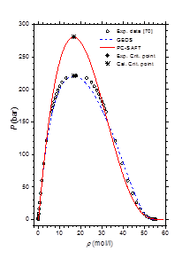
Figure 1 Pressure-density diagram of water at saturated liquid and vapor phases.
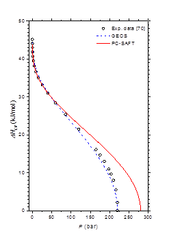
Figure 2 Molar enthalpy of vaporization of water from triple to critical points.

Vapor-liquid phase behavior of methylamine/water mixture

A bank of N = 183 bibliographical experimental vapor-liquid phase equilibria data for the methylamine/water (Temperature range: 251−423 K and pressure range: 0.009−28.72 bar) has been constituted and exploited to deduce the binary cross-interaction parameters in the PC-SAFT and GEOS equations of state. The same FORTRAN program is used for the calculation of the two-phase vapor-liquid equilibria and the regression of the adjustable binary cross-interaction parameters. For a binary mixture, at fixed values of temperature T and mole fraction of the liquid phase x (or the vapor phase y), the vapor pressure P and molar composition of the vapor phase y (or the liquid phase x), as well as the saturated liquid molar density and the saturated vapor molar density  are computed by solving a set of 4 algebraic equations (2 chemical potential and 2 pressure equalities). The binary cross-interaction parameters are determined by the minimization of the relative difference between literature data and theoretical values of vapor pressure and vapor mole composition:

S 2 = j=1 N [ ( P j exp P j cal P j exp ) 2 + w i ( y j exp y j cal y j exp ) 2 ] MathType@MTEF@5@5@+= feaagKart1ev2aqatCvAUfeBSjuyZL2yd9gzLbvyNv2CaerbuLwBLn hiov2DGi1BTfMBaeXatLxBI9gBaerbd9wDYLwzYbItLDharqqtubsr 4rNCHbGeaGqiVCI8FfYJH8YrFfeuY=Hhbbf9v8qqaqFr0xc9pk0xbb a9q8WqFfeaY=biLkVcLq=JHqpepeea0=as0Fb9pgeaYRXxe9vr0=vr 0=vqpWqaaeaabiGaciaacaqabeaadaqaaqaaaOqaaKqzGeaeaaaaaa aaa8qacaWGtbqcfa4damaaBaaaleaajugWa8qacaaIYaaal8aabeaa jugib8qacqGH9aqpjuaGdaGfWbGcbeWcpaqaaKqzadWdbiaadQgacq GH9aqpcaaIXaaal8aabaqcLbmapeGaamOtaaqdpaqaaKqzGeWdbiab ggHiLdaajuaGdaWadaGcpaqaaKqba+qadaqadaGcpaqaaKqba+qada WcaaGcpaqaaKqzGeWdbiaadcfal8aadaqhaaqaaKqzadWdbiaadQga aSWdaeaajugWa8qacaWGLbGaamiEaiaadchaaaqcLbsacqGHsislca WGqbWcpaWaa0baaeaajugWa8qacaWGQbaal8aabaqcLbmapeGaam4y aiaadggacaWGSbaaaaGcpaqaaKqzGeWdbiaadcfal8aadaqhaaqaaK qzadWdbiaadQgaaSWdaeaajugWa8qacaWGLbGaamiEaiaadchaaaaa aaGccaGLOaGaayzkaaqcfa4damaaCaaaleqabaqcLbsapeGaaGOmaa aacqGHRaWkcaWG3bqcfa4damaaBaaaleaajugib8qacaWGPbaal8aa beaajuaGpeWaaeWaaOWdaeaajuaGpeWaaSaaaOWdaeaajugib8qaca WG5bWcpaWaa0baaeaajugWa8qacaWGQbaal8aabaqcLbmapeGaamyz aiaadIhacaWGWbaaaKqzGeGaeyOeI0IaamyEaSWdamaaDaaabaqcLb mapeGaamOAaaWcpaqaaKqzadWdbiaadogacaWGHbGaamiBaaaaaOWd aeaajugib8qacaWG5bWcpaWaa0baaeaajugWa8qacaWGQbaal8aaba qcLbmapeGaamyzaiaadIhacaWGWbaaaaaaaOGaayjkaiaawMcaaSWd amaaCaaabeqaaKqzadWdbiaaikdaaaaakiaawUfacaGLDbaaaaa@89AE@ (44)

whereN is the number of experimental data used in the regression and wi is a weighting coefficient for the relative deviations of the molar vapor composition. Regardless of the type of the experimental data, wi = 0 when only (T,P,x) or (T,P,y) values are available and wi = 1 when (T,P,x,y) values are available.

The optimized values of the binary cross-interaction parameters along with the absolute average deviations AAD for (1) vapor pressures (ΔP) and (2) molar compositions of the vapor phase are given in Table 4 for both thermodynamic models. As can be observed, the two equations of state correlate similarly the vapor pressure data. However, the GEOS (Δy = 0.6%) reproduces more accurately the molar composition data of the vapor phase than the PC-SAFT (Δy = 1.2%). In Figure 3 & Figure 4 are depicted the P-T curves of methylamine/water system at different values of the molar and mass fractions (Oldham or Dühring diagrams), respectively. As can be noted, both equations of state correlate comparably well the experimental data. The partial pressures of methylamine are estimated by the two investigated equations of state and compared to the experimental counterpart,41 as illustrated in Figure 5. Both models give globally similar predictions of partial pressures with a slight superiority to the GEOS equation of state.


          K ij MathType@MTEF@5@5@+= feaagKart1ev2aaatCvAUfeBSjuyZL2yd9gzLbvyNv2CaerbuLwBLn hiov2DGi1BTfMBaeXatLxBI9gBaerbd9wDYLwzYbItLDharqqtubsr 4rNCHbGeaGqiVCI8FfYJH8YrFfeuY=Hhbbf9v8qqaqFr0xc9pk0xbb a9q8WqFfeaY=biLkVcLq=JHqpepeea0=as0Fb9pgeaYRXxe9vr0=vr 0=vqpWqaaeaabiGaciaacaqabeaadaqaaqaaaOqaaKqzGeGaam4saO WaaSbaaSqaaiaadMgacaWGQbaabeaaaaa@395D@

  λ ij MathType@MTEF@5@5@+= feaagKart1ev2aaatCvAUfeBSjuyZL2yd9gzLbvyNv2CaerbuLwBLn hiov2DGi1BTfMBaeXatLxBI9gBaerbd9wDYLwzYbItLDharqqtubsr 4rNCHbGeaGqiVCI8FfYJH8YrFfeuY=Hhbbf9v8qqaqFr0xc9pk0xbb a9q8WqFfeaY=biLkVcLq=JHqpepeea0=as0Fb9pgeaYRXxe9vr0=vr 0=vqpWqaaeaabiGaciaacaqabeaadaqaaqaaaOqaaKqzGeGaeq4UdW wcfa4aaSbaaeaajugWaiaadMgacaWGQbaajuaGbeaaaaa@3C76@

ν ij MathType@MTEF@5@5@+= feaagKart1ev2aaatCvAUfeBSjuyZL2yd9gzLbvyNv2CaerbuLwBLn hiov2DGi1BTfMBaeXatLxBI9gBaerbd9wDYLwzYbItLDharqqtubsr 4rNCHbGeaGqiVCI8FfYJH8YrFfeuY=Hhbbf9v8qqaqFr0xc9pk0xbb a9q8WqFfeaY=biLkVcLq=JHqpepeea0=as0Fb9pgeaYRXxe9vr0=vr 0=vqpWqaaeaabiGaciaacaqabeaadaqaaqaaaOqaaKqzGeGaeqyVd4 wcfa4aaSbaaeaajugWaiaadMgacaWGQbaajuaGbeaaaaa@3C7A@

ΔP

Δy

T range

N

Ref.

EoS

K 12 MathType@MTEF@5@5@+= feaagKart1ev2aaatCvAUfeBSjuyZL2yd9gzLbvyNv2CaerbuLwBLn hiov2DGi1BTfMBaeXatLxBI9gBaerbd9wDYLwzYbItLDharqqtubsr 4rNCHbGeaGqiVCI8FfYJH8YrFfeuY=Hhbbf9v8qqaqFr0xc9pk0xbb a9q8WqFfeaY=biLkVcLq=JHqpepeea0=as0Fb9pgeaYRXxe9vr0=vr 0=vqpWqaaeaabiGaciaacaqabeaadaqaaqaaaOqaaKqzGeGaam4saK qbaoaaBaaaleaajugWaiaaigdacaaIYaaaleqaaaaa@3AB4@

K 2 1 MathType@MTEF@5@5@+= feaagKart1ev2aaatCvAUfeBSjuyZL2yd9gzLbvyNv2CaerbuLwBLn hiov2DGi1BTfMBaeXatLxBI9gBaerbd9wDYLwzYbItLDharqqtubsr 4rNCHbGeaGqiVCI8FfYJH8YrFfeuY=Hhbbf9v8qqaqFr0xc9pk0xbb a9q8WqFfeaY=biLkVcLq=JHqpepeea0=as0Fb9pgeaYRXxe9vr0=vr 0=vqpWqaaeaabiGaciaacaqabeaadaqaaqaaaOqaaKqzGeGaam4saS WaaSbaaWqaamaaBaaabaGaaGOmaaqabaWaaSbaaeaacaaIXaaabeaa aeqaaaaa@393B@


(%)

(%)

(K)


PC-SAFT

-0.10765

-0.31874


9.08

1.22

256−423

183

40–51

GEOS

 0.08254

-0.20682

0.14827

-0.03583

9.38

0.60

256−423

183

40–51

Table 4 Binary cross-interaction parameters for the PC-SAFT and GEOS equations of state
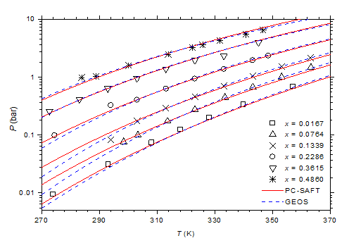
Figure 3 P-T-x diagram of methylamine/water mixture. Comparison of experimental data41 to calculated curves with GEOS and PC-SAFT models.
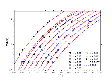
Figure 4 P-T-ξ diagram of methylamine/water mixture. Comparison of experimental data40 to calculated values with GEOS and PC-SAFT models.
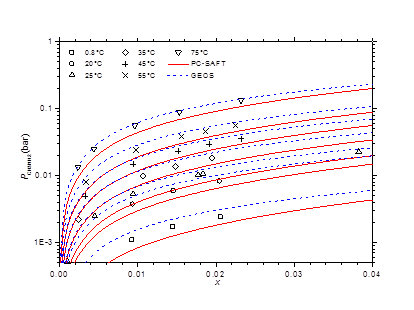
Figure 5 Partial pressures of methylamine via molar liquid fraction at different isotherms. Comparison of experimental data41 to theoretical values with GEOS and PC-SAFT.

The isobaric vapor-liquid phase equilibrium diagram at atmospheric pressure is illustrated in Figure 6. It is found that the theoretical curves of both EOS are very similar and reproduce with good accuracy the experimental dew point data in the entire composition range. However, the experimental bubble point data are offset from the calculated curves for molar liquid fractions lower than 0.2. The vapor-liquid phase equilibrium isotherms at different temperatures in the range of 303-383 K are illustrated in Figure 7-9. It can be concluded that the two models are similar and reproduce well the experimental data. A slight superiority is noted for the GEOS equation of state at high temperatures (near the critical temperature of methylamine) as can be seen for the isotherm 383.15 K for example. The enthalpy-composition-temperature (h-ξ-T) diagram of the saturated liquid phase of the methylamine/water system is represented in Figure 10. The predicted curves by the PC-SAFT and GEOS equations of state are confronted to literature data.40 It can be observed that the two investigated models reproduce satisfactorily well the available experimental data in the literature. Finally, it can be concluded that both investigated EOS, GEOS and PC-SAFT, are in general similar and correlate with the same order of precision the experimental data of the methylamine/water binary mixture. It should be noted however that the available bibliographical data contain only a few data in the vicinity of the critical region where the capacity of each model to correlate the vapor-liquid phase behavior can be appreciated.
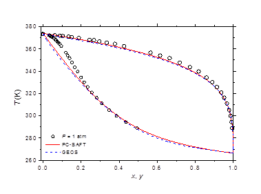
Figure 6 Vapor-liquid phase equilibria at atmospheric pressure of methylamine/water. Comparison of experimental data49  to theoretical curves with GEOS and PC-SAFT models.
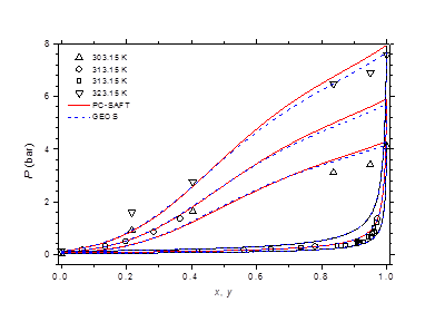
Figure 7 Phase equilibria of methylamine/water at 303.15, 313.15 and 323.15 K. Comparison of experimental data50,51 to calculated curves with GEOS and PC-SAFT.
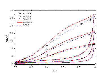
Figure 8 Phase equilibria of methylamine/water at 343.15, 363.15 and 383.15 K. Comparison of experimental data50 to calculated curves with GEOS and PC-SAFT.
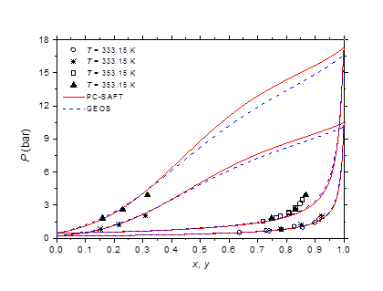
Figure 9 Phase behavior of methylamine/water at 333.15 and 353.15 K. Comparison of experimental data 51 to calculated curves with GEOS and PC-SAFT.
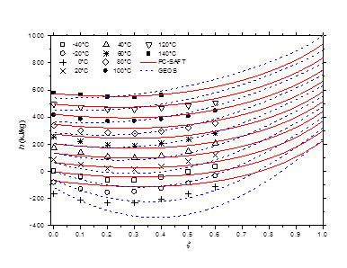
Figure 10 h-ξ-T diagram of saturated liquid phase for methylamine/water mixture. Comparison of literature data40 to calculated curves by GEOS and PC-SAFT.

Summary

When the two investigated thermodynamic models for water-methylamine system property and liquid-vapor phase calculations are compared, it is found that

  1. the performances of both equations of state in predicting the mixture properties are comparable;
  2. GEOS is more accurate in reproducing and predicting the pure fluid properties and liquid-vapor phase equilibria of water and methylamine
  3. GEOS is much easier in use and handier than the complex and more elaborated PC-SAFT equation of state. This issue is very important for the praxis, in particular if the equation of state is to be implemented in sophisticated flow-sheeting software.

For all these reasons, solely GEOS is retained in the following for the prediction of the properties of the binary mixtures of methylamine and water (Tables in Appendices C.1 and C2 and Figure 11 & Figure 12 representing the (h-T) and (s-T) diagrams of the saturated methylamine/water mixture up to very high temperature and pressure, respectively). It must be noted however that these curves and tables are deduced by extrapolation outside the domain of the available bibliographical data. Reasonable results are obtained, however the prediction accuracy in these areas is unknown. More experimental data are needed to assess the quality of the predicted properties, particularly in the critical and single-phase regions.

Figure 11 h-T-ξ diagram of saturated methylamine/water mixture plotted with GEOS.

Figure 12 s-T-ξ diagram of saturated methylamine/water mixture plotted with GEOS.

Conclusion

The vapor-liquid phase equilibria and thermodynamic properties of the methylamine/water binary mixture are modeled using two approaches, PC-SAFT equation of state and GEOS. A confrontation of the calculated and experimental data for pure fluids shows that the GEOS model is more accurate than the PC-SAFT equation in reproducing the vapor-liquid phase behavior and molar enthalpy of vaporization in the vicinity of the critical point of pure water. The binary cross-interaction parameters in the equations of state for the mixture are fitted from the few available vapor-liquid equilibria data. The comparison of the theoretical property predictions with experimental data leads to the conclusion that the two investigated equations of state are in general comparable in the calculation of the two-phase behavior of the methylamine/water system. However, the general cubic equation of state GEOS is more accurate in the neighborhood of the critical temperature of methylamine. This fact is probably due to the more accurate description of the vapor-liquid equilibrium of pure components near the critical region by GEOS. Further, a practical advantage of this equation of state is its simple mathematical structure, more tractable and easier to apply than the complex PC-SAFT EOS.

Acknowledgements

None.

Conflict of interest

The author declares that there is no conflict of interest.

References

  1. Tyagi KP. Ammonia-salts vapor absorption refrigeration systems. Journal of Heat Recovery Systems. 1984;4(6)4:427–431.
  2. Darwish NA, Al Hashimi SH, Al Mansoori AS. Performance analysis and evaluation of a commercial absorption–refrigeration water–ammonia (ARWA) system. International Journal of Refrigeration. 2008;31(7) 31:1214–1223.
  3. Zavaleta Aguilar EW, Simões Moreira JR. Thermal design of a tray-type distillation column of an ammonia/water absorption refrigeration cycle. Applied Thermal Engineering. 2012;41(1):52–60.
  4. Fernández Seara J, Sieres J. The importance of the ammonia purification process in ammonia–water absorption systems. Energy Conversion and Management. 2006;47(13-14):1975–1987.
  5. Horuz I, Callander TM. Experimental investigation of a vapor absorption refrigeration system. International Journal of Refrigeration. 2004;27(1):10–16.
  6. Eicker U, Pietruschka D. Design and performance of solar powered absorption cooling systems in office buildings. Energy and Buildings. 2009;41:81–91.
  7. Engler M, Grossman G, Hellmann HM. Comparative simulation and investigation of ammonia-water: absorption cycles for heat pump applications. International Journal of Refrigeration. 1997;20(7):504–516.
  8. Siddiqui MU, Said SA. A review of solar powered absorption systems. Renewable and Sustainable Energy Reviews. 2015;42:93–115.
  9. Ullah K, Saidur R, Ping H, et al. A review of solar thermal refrigeration and cooling methods. Renewable and Sustainable Energy Reviews. 2013;24:499–513.
  10. Wu W, Wang B, Shi W, et al. An overview of ammonia-based absorption chillers and heat pumps. Renewable and Sustainable Energy Reviews. 2014;31:681–707.
  11. Steiu S, Salavera D, Bruno JC, et al. A basis for the development of new ammonia–water–sodium hydroxide absorption chillers. International Journal of Refrigeration. 2009;32(4):577–587.
  12. Balamuru VG, Ibrahim OM, Barnett SM. Simulation of ternary ammonia–water–salt absorption refrigeration cycles. International Journal of Refrigeratio.2000;23(1):31–42.
  13. Sun DW. Comparison of the performances of NH3-H2O, NH3-LiNO3 and NH3-NaSCN absorption refrigeration systems. Energy Conversion and Management. 1998;39(5-6):357–368.
  14. Zhu L, Wang S, Gu J. Performance investigation of a thermal-driven refrigeration system. International Journal of Energy Research. 2008;32(10):939–949.
  15. Chekir N, Mejbri Kh, Bellagi A. Simulation of an absorption chiller operating with alkane mixtures. International Journal of Refrigeration. 2006;29(10):469–475.
  16. Kaushik SC, Kumar R. Comparative study of an absorber heat recovery cycle for solar refrigeration using NH3 refrigerant with liquid/solid absorbents. International Journal of Energy Research. 1987;11(1):123–132.
  17. Ahachad M, Charia M, Bernatchou A. Study of an improved NH3/H2O solar absorption refrigerating machine in Rabat (Morocco). Solar Energy Materials and Solar Cells.1992;28(1):71–79.
  18. Lazzarin RM, Gasparella A, Longo GA. Ammonia-water absorption machines for refrigeration: theoretical and real performances. International Journal of Refrigeration.1996;19(4):239–246.
  19. Ghaddar NK, Shihab M, Bdeir F. Modeling and simulation of solar absorption system performance in Beirut. Renewable Energy. 1997;10(4):539–558.
  20. Joudi KA, Lafta AH. Simulation of a simple absorption refrigeration system. Energy Conversion and Management. 2001;42(13):1575–1605.
  21. Florides GA, Kalogirou SA, Tassou SA, et al. Modeling and simulation of an absorption solar cooling system for Cyprus. Solar Energy. 2002;72(1):43–51.
  22. Barragán RM, Heard CL, Arellano VM, et al. Experimental performance of the water/calcium chloride system in a heat transformer. International Journal of Energy Research.1996; 20(8):651–661.
  23. Ma X, Chen J, Li S, et al. Application of absorption heat transformer to recover waste heat from a synthetic rubber plant. Applied Thermal Engineering.2003;23(7):797–806.
  24. Horuz I, Kurt B. Absorption heat transformers and an industrial application. Renewable Energy. 2010;35(10):2175–2181.
  25. Rivera W, Huicochea A, Martínez H, et al. Exergy analysis of an experimental heat transformer for water purification. Energy. 2011;36(1):320–327.
  26. Sekar S, Saravanan R. Experimental studies on absorption heat transformer coupled distillation system. Desalination. 2011;274(1-3):292–301.
  27. Huicochea A, Rivera W, Martínez H, et al. Analysis of the behavior of an experimental absorption heat transformer for water purification for different mass flux rates in the generator. Applied Thermal Engineering. 2013;52(1):38–45.
  28. Ibarra Bahena J, Romero RJ, Velazquez Avelar L, et al. Experimental thermodynamic evaluation for a single stage heat transformer prototype build with commercial PHEs. Applied Thermal Engineering. 2015;75:1262–1270.
  29. Srikhirin P, Aphornratana S, Chungpaibulpatana S. A review of absorption refrigeration technologies. Renewable and Sustainable Energy Reviews. 2001;5(4):343–372.
  30. Holmberg P, Berntsson T. Alternative working fluids in heat transformers. A shrae Transactions.1990:96.
  31. Abed AM, Alghoul MA, Sopian K, et al. Enhancement aspects of single stage absorption cooling cycle: A detailed review. Renewable and Sustainable Energy Reviews. 2017;77(C):1010-1045.
  32. Kilic M, Kaynakli O. Second law-based thermodynamic analysis of water-lithium bromide absorption refrigeration system. Energy. 2007;32(8):1505–1512.
  33. Palacios Bereche R, Gonzales R, Nebra SA. Exergy calculation of lithium bromide–water solution and its application in the exergetic evaluation of absorption refrigeration systems LiBr-H2O. International Journal of Energy Research. 2012;36(2):166–181.
  34. Misra RD, Sahoo PK, Sahoo S, et al. Thermo-economic optimization of a single effect water/LiBr vapor absorption refrigeration system. International Journal of Refrigeration. 2003;26(2):158–169.
  35. Uemura T, Higuchi Y, Hasaba S. Studies on the monomethylamine–water absorption refrigerating machine. Refrigeration. 1967;42(471):2–13.
  36. Tyagi KP. Comparison of binary mixtures for absorption refrigeration systems. Heat Recovery Systems.1983;3(5):421-429.
  37. Pilatowsky I, Rxver W, Best R, et al. Thermodynamic design data for absorption heat pump systems operating on monomethylamine-water. Part III: Simultaneous cooling and heating. Heat Recovery Systems &CHP. 1995;15(6):583-589.
  38. Pilatowsky I, Rivera W, Romero RJ. Thermodynamic analysis of monomethylamine–water solutions in a single-stage solar absorption refrigeration cycle at low generator temperatures. Solar Energy Materials & Solar Cells. 2001;70(3):287–300.
  39. Pilatowsky I, Rivera W, Romero JR. Performance evaluation of a monomethylamine–water solar absorption refrigeration system for milk cooling purposes. Applied Thermal Engineering. 2004;24(7):1103–1115.
  40. Romero RJ, Luis Guillen, Pilatowsky I. Monomethylamine–water vapor absorption refrigeration system. Applied Thermal Engineering. 2005;25:867–876.
  41. Felsing WA, Thomas A. Vapor pressures and other physical constants of methylamine and methylamine solutions. Ind. Eng. Chem. 1929;21(12):1269-1272.
  42. Felsing WA, Wohlford PH. The heats of solution of gaseous methylamine. Journal of American Chemical Society. 1932;54(4):1442–1445.
  43. Mehl W, Ein Ubersichtsdiagramm log p-1/T fur das paar MethylaminWasser. Zeitsch f Ges. Kalte-Industrie. 1935;42(1):13–25.
  44. Bonauguri EA, Bonfanti A, Gurdjian V. Gemische von CH2NH3 und H2O. La Thermotecnia.1954;5:53–78.
  45. Ehmke HJ. Dissertation universitit essen. Forschungbericht des DKV No.1984.
  46. Roberson JP, Lee CY, Squires RG, et al. Vapor pressure of ammonia and monomethylamine in solutions for absorption refrigeration systems. ASHRAE Trans. 1966;72(1):198–208.
  47. Uemura T, Higuchi Y, Saito Y, et al. Studies on the Mono-Methylamine-Water Absorption Refrigerating Machine. Refrigeration. 1967;(42)471:2-13.
  48. Pilatowsky I, Rivera W, Best R. State equations for monomethylamine–water solutions, derived from equilibrium diagrams. Non-published internal report. No. LES 94-0504-104. Mexico: Energy Solar Laboratory; IIM-UNAM; 1994. 110 p.
  49. Gao D, Qiu Z, Yu S. Vapor-liquid equilibrium of three binary system: monomethylamine-H2O: dimethylamine-H2O and trimethylamine-H2O. Nanchang Daxue Xuebao. 2003;137(3):69–72.
  50. Xu X, An L, Zheng G. Measurement of Vapor-Liquid Equilibrium Data for Products in Methanol Amination. Gaoxiao Huaxue Gongcheng Xuebao. 1995;9(1):97–105.
  51. Stumm F, Heintz A, Lichtenthaler RN. Experimental data and modeling of vapor-liquid equilibria of the ternary system carbon dioxide + water + methylamine at 313, 333 and 353 K and pressures up to 0.4 MPa. Fluid Phase Equilibria. 1993;91(2):331–348.
  52. Huang S, Radosz M. Equation of state for small, large, pollydisperse and associationg molecules. Industrial Engineering Chemical Research. 1990;29(11):2284–2294.
  53. Huang S, Radosz M. Equation of state for small, large, pollydisperse and associationg molecules: extention to fluid mixtures. Industrial Engineering Chemical Research. 19991;30(8):1994–2005.
  54. Gross J, Sadowski G. Application of the perturbed theory to a hard-chainreference fluid: an equation of state for square-well chains. Fluid Phase Equilibria. 2000;168(2):183–199.
  55.  Gross J, Sadowski G. Perturbed-Chain SAFT: an equation of state based on a perturbation theory for chain molecules. Industrial Engineering Chemical Research. 20001;40(4):1244–1260.
  56. Gross J, Sadowski G. Application of the perturbed-chain SAFT equation of state to associating systems, Industrial Engineering Chemical Research. 2002;41(22):5510–5515.
  57. Gross J, Sadowski G. Modeling Polymer Systems Using the Perturbed-Chain Statistical Associating Fluid Theory Equation of State. Industrial Engineering Chemical Research. 2002;41(5):1084–1093.
  58. Gross J, Spuhl O, Tumakaka F, et al. Modeling Copolymer Systems Using the Perturbed-Chain SAFT Equation of State. Industrial Engineering Chemical Research. 2003;42(6):1266–1274.
  59. Mejbri KH, Thesis. Study of a single-pressure absorption refrigeration cycle: modeling, simulation and thermohydraulic design of a pilot installation for solar cold production. Tunisia: National Engineers School of Monastir; 2008. 6 p.
  60. Mejbri Kh, Bellagi A. Équation d’état PC-SAFT appliquée aux fluides purs et aux mélanges binaires. Journal de la Société Chimique de Tunisie. 2005;7:125–138.
  61. Mejbri Kh, Bellagi A. Modeling of the thermodynamic properties of the water/ammonia mixture by three different approaches. International Journal of Refrigeration. 2006;29(2):211–218.
  62. Mejbri Kh, Taieb A, Bellagi A. Phase equilibria calculation of binary and ternary mixtures of associating fluids applying PC-SAFT equation of state. Journal of Supercritical Fluids. 2015;104(10):132–144.
  63. Feroiu V, Geană D. Computation of vapor-liquid equilibrium in N2 + CO2 + CH4 system by a general cubic equation of state. Fluid Phase Equilibria. 1990;55(2):263–270.
  64. Geană D, Feroiu V. Calculation of Joule-Thomson inversion curves from a general cubic equation of state. Fluid Phase Equilibria. 1992;77(1):121–132.
  65. Geană D, Feroiu V. Thermodynamic properties of pure fluids using the GEOS3C equation of state. Fluid Phase Equilibria. 2000;174(1):51–68.
  66. Feroiu V, Geană D. Volumetric and thermodynamic properties for pure refrigerants and refrigerant mixtures from cubic equations of state. Fluid Phase Equilibria. 2003;207(1-2):283–300.
  67. Secuianu C, Feroiu V, Geană D. Phase behavior for carbon dioxide+ethanol system: Experimental measurements and modeling with a cubic equation of state. Journal of Supercritical Fluids. 2008;47(2):109–116.
  68. Boggs p, Byrd R, Rogers J, et al. ODRPACK version 2.01 Software for weighted orthogonal distance regression, NIST. USA: Interagency Report; 1992. 120 p.
  69. Shacham M. Numerical solution of constrained nonlinear equations. International Journal of Numerical Methods in Engineering. 1986;23(8):1455–1481.
  70. NIST Standard Reference Database. In: Linstrom PJ, Mallard WG, editors. 2011.
  71. Tyagi KP. Methylamine–sodium thiocyanate vapor absorption refrigeration. Heat Recovery Systems & CHP. 1992;12(3):283-287.
  72. Vargraftik NB, Vinoradov YK, Yargin VS. Handbook of Physical Properties of Liquids and Gases, Pure Substances and Mixtures. Third Augmented and Revised Edition. New York: Begellhouse inc; 1996. 1359 p.
  73. Perry RH, Green DW, Maloney JO. Perry’s Chemical Engineers’ Handbook. 7th edition. Newyork: McGraw-Hill; 1997. 2641 p.
Creative Commons Attribution License

©2018 Mejbri, et al. This is an open access article distributed under the terms of the, which permits unrestricted use, distribution, and build upon your work non-commercially.