Submit manuscript...
eISSN: 2469-2778

Hematology & Transfusion International Journal

Research Article Volume 11 Issue 1

Comparative study between a deterministic and stochastic model´s for the hematopoietic reconstitution

Miguel Ángel Martínez Hernández, Dennis Lumpuy Obregón

Universidad Central “Marta Abreu” de Las Villas, Santa Clara, Cuba

Correspondence: Miguel Ángel Martínez Hernández, Universidad Central “Marta Abreu” de Las Villas, Santa Clara, Villa Clara, Cuba

Received: October 17, 2022 | Published: January 26, 2023

Citation: Hernández MAM, Obregón DL. Comparative study between a deterministic and stochastic model´s for the hematopoietic reconstitution. Hematol Transfus Int. 2023;11(1):10-14. DOI: 10.15406/htij.2023.11.00293

Download PDF

Abstract

The dynamics of the processes of cell maturation and regeneration is a branch currently in development for medicine, so taking advantage of the facilities of mathematics to model and solve environmental problems, different models of differential equations have been developed to describe these processes. From the existing deterministic models, the particular case of the hematopoietic cell is chosen, for of a comparative study on the influence of the medium on the process of cell maturation. For this, a probabilistic model of differential equations with six compartments is used. The stochastic term or environmental noise in this particular case modeled by a Weiner process. The inclusion of this term makes it possible to perform an analysis conditioned on the influence of the medium of the different processes of cellular maturation, in this case, of the hematopoietic cell. It is established that the stochastic model reflects a more precise approach to the clinical data used.

Keywords: deterministic models, hematopoietic cell, cell maturation, stochastic model

Introduction

Stem cells are cells that have the ability to continually renew themselves by successive divisions and to specialize (differentiate) and become many types of body cells and, therefore, produce cells from one or several perfectly functional tissues. Stem cells can be divided without losing their properties, so that in most of the tissues of an adult there are populations of stem cells that, when divided, renew dead cells and regenerate damaged tissues. When a stem cell divides, each new cell can remain a stem cell or become another type of cell with a more specialized function, such as a muscle cell, a red blood cell or a heart cell.

The possibility to maintain in a culture stem cells for long periods of time (especially embryonic ones) and to differentiate into different types of cells, allows them to be used in regenerative medicine, in order to replace damaged tissues with degenerative lesions or diseases.

Due to the growing interest in stem cell applications, such as stem cell-based therapies for damaged organs, degenerative diseases1 or reconstitution of the blood structure after chemotherapy in the treatment of leukemia,2 a broad spectrum of methods has been developed to expand knowledge about the rules of this process. Several mathematical models were developed to aid in the understanding of stem cell differentiation.3–7 The models involve different mathematical approaches to describe the processes of differentiation and self-renewal7,8–10 that involve the proliferation of stem cells3 and the mechanisms of differentiation at each stage.4 All these models describe different parts of the homeostasis process in adult tissue. These models represent a first deterministic approach to mathematically understand this complex dynamic. Another important aspect in mathematical modeling is to incorporate those environmental and external disturbances into the system, which in the previous models are not considered, but which nonetheless positively or negatively influence the maturation and self-renewal process of the stem cells. This gives rise to stochastic models that, as a fundamental characteristic, consider the environmental disturbances of the system, which are expressed mathematically by means of diffusion coefficients and gaussian noise. These new factors considered has a direct impact on the modeling and representation of the cell maturation process. The development and study of this type of models expresses the existing interest in deepening knowledge in the applications that the area of ​​stochastic processes has to biology. Hence, in this investigation our scientific problem derives from the interpretation of this random noise in the process of cellular maturation.

Material and methods

The model is based on the assumption that the differentiation process is strictly related to cell division, that is, that differentiation takes place only during cell division, then the rate of cell differentiation is proportional to that of proliferation.

To quantitatively describe the self-renewal, the so-called self-renewal fraction is introduced, a i MathType@MTEF@5@5@+= feaagKart1ev2aaatCvAUfeBSjuyZL2yd9gzLbvyNv2CaerbuLwBLn hiov2DGi1BTfMBaeXatLxBI9gBaerbd9wDYLwzYbItLDharqqtubsr 4rNCHbGeaGqkY=Mj0xXdbba91rFfpec8Eeeu0xXdbba9frFj0=OqFf ea0dXdd9vqaq=JfrVkFHe9pgea0dXdar=Jb9hs0dXdbPYxe9vr0=vr 0=vqpWqaaeaabiGaciaacaqabeaadaqaaqaaaOqaaiaadggadaWgaa WcbaGaamyAaaqabaaaaa@390E@ , which describes which fraction of progeny cells (offspring) is identical to the progenitor cells, were i=1,...,n MathType@MTEF@5@5@+= feaagKart1ev2aaatCvAUfeBSjuyZL2yd9gzLbvyNv2CaerbuLwBLn hiov2DGi1BTfMBaeXatLxBI9gBaerbd9wDYLwzYbItLDharqqtubsr 4rNCHbGeaGqkY=Mj0xXdbba91rFfpec8Eeeu0xXdbba9frFj0=OqFf ea0dXdd9vqaq=JfrVkFHe9pgea0dXdar=Jb9hs0dXdbPYxe9vr0=vr 0=vqpWqaaeaabiGaciaacaqabeaadaqaaqaaaOqaaiaadMgacqGH9a qpcaaIXaGaaiilaiaac6cacaGGUaGaaiOlaiaacYcacaWGUbaaaa@3E26@  is the corresponding stage of the maturation process (this parameter can be interpreted as the probability that the daughter cell has the same properties as the stem cell). Furthermore, p i MathType@MTEF@5@5@+= feaagKart1ev2aaatCvAUfeBSjuyZL2yd9gzLbvyNv2CaerbuLwBLn hiov2DGi1BTfMBaeXatLxBI9gBaerbd9wDYLwzYbItLDharqqtubsr 4rNCHbGeaGqkY=Mj0xXdbba91rFfpec8Eeeu0xXdbba9frFj0=OqFf ea0dXdd9vqaq=JfrVkFHe9pgea0dXdar=Jb9hs0dXdbPYxe9vr0=vr 0=vqpWqaaeaabiGaciaacaqabeaadaqaaqaaaOqaaiaadchadaWgaa WcbaGaamyAaaqabaaaaa@391D@  for i=1,...,n1 MathType@MTEF@5@5@+= feaagKart1ev2aaatCvAUfeBSjuyZL2yd9gzLbvyNv2CaerbuLwBLn hiov2DGi1BTfMBaeXatLxBI9gBaerbd9wDYLwzYbItLDharqqtubsr 4rNCHbGeaGqkY=Mj0xXdbba91rFfpec8Eeeu0xXdbba9frFj0=OqFf ea0dXdd9vqaq=JfrVkFHe9pgea0dXdar=Jb9hs0dXdbPYxe9vr0=vr 0=vqpWqaaeaabiGaciaacaqabeaadaqaaqaaaOqaaiaadMgacqGH9a qpcaaIXaGaaiilaiaac6cacaGGUaGaaiOlaiaacYcacaWGUbGaeyOe I0IaaGymaaaa@3FCE@  is the population proliferation rate in stage i, μ i , α i ( W 1,t ,... W n,t ) c 1 >0 i1 μ i == μ n1 =0 μ n >0 a 1 > 1 2 a 1 > a i i=2,...,n1 n=6 MathType@MTEF@5@5@+= feaagKart1ev2aaatCvAUfeBSjuyZL2yd9gzLbvyNv2CaerbuLwBLn hiov2DGi1BTfMBaeXatLxBI9gBaerbd9wDYLwzYbItLDharqqtubsr 4rNCHbGeaGqkY=Mj0xXdbba91rFfpec8Eeeu0xXdbba9frFj0=OqFf ea0dXdd9vqaq=JfrVkFHe9pgea0dXdar=Jb9hs0dXdbPYxe9vr0=vr 0=vqpWqaaeaabiGaciaacaqabeaadaqaaqaaaOabaeqabaGaamyAai aacYcacqaH8oqBdaWgaaWcbaGaamyAaaqabaGccaGGSaaabaGaeqyS de2aaSbaaSqaaiaadMgaaeqaaaGcbaWaaeWaaeaacaWGxbWaaSbaaS qaaiaaigdacaGGSaGaamiDaaqabaGccaGGSaGaaiOlaiaac6cacaGG UaGaam4vamaaBaaaleaacaGGUbGaaiilaiaadshaaeqaaaGccaGLOa GaayzkaaaabaGabm4yayaafaWaaSbaaSqaaiaaigdaaeqaaOGaeyOp a4JaaGimaaqaaiaadMgacqGHsislcaaIXaaabaGaeqiVd02aaSbaaS qaaiaadMgaaeqaaOGaeyypa0JaeS47IWKaeyypa0JaeqiVd02aaSba aSqaaiaad6gacqGHsislcaaIXaaabeaakiabg2da9iaaicdaaeaacq aH8oqBdaWgaaWcbaGaamOBaaqabaGccqGH+aGpcaaIWaaabaGaamyy amaaBaaaleaacaaIXaaabeaakiabg6da+maalaaabaGaaGymaaqaai aaikdaaaaabaGaamyyamaaBaaaleaacaaIXaaabeaakiabg6da+iaa dggadaWgaaWcbaGaamyAaaqabaaakeaacaWGPbGaeyypa0JaaGOmai aacYcacaGGUaGaaiOlaiaac6cacaGGSaGaamOBaiabgkHiTiaaigda aeaacaWGUbGaeyypa0JaaGOnaaaaaa@773D@  for i=1,...,n MathType@MTEF@5@5@+= feaagKart1ev2aaatCvAUfeBSjuyZL2yd9gzLbvyNv2CaerbuLwBLn hiov2DGi1BTfMBaeXatLxBI9gBaerbd9wDYLwzYbItLDharqqtubsr 4rNCHbGeaGqkY=Mj0xXdbba91rFfpec8Eeeu0xXdbba9frFj0=OqFf ea0dXdd9vqaq=JfrVkFHe9pgea0dXdar=Jb9hs0dXdbPYxe9vr0=vr 0=vqpWqaaeaabiGaciaacaqabeaadaqaaqaaaOqaaiaadMgacqGH9a qpcaaIXaGaaiilaiaac6cacaGGUaGaaiOlaiaacYcacaWGUbaaaa@3E26@  represents the death rate in stage i and c i t MathType@MTEF@5@5@+= feaagKart1ev2aaatCvAUfeBSjuyZL2yd9gzLbvyNv2CaerbuLwBLn hiov2DGi1BTfMBaeXatLxBI9gBaerbd9wDYLwzYbItLDharqqtubsr 4rNCHbGeaGqkY=Mj0xXdbba91rFfpec8Eeeu0xXdbba9frFj0=OqFf ea0dXdd9vqaq=JfrVkFHe9pgea0dXdar=Jb9hs0dXdbPYxe9vr0=vr 0=vqpWqaaeaabiGaciaacaqabeaadaqaaqaaaOqaaiaadogadaWgaa WcbaGaamyAaaqabaGccaWG0baaaa@3A13@  represent the population density in the corresponding stage on the time .

Then:

{ d C 1 ( t ) dt = f 1 ( s(t), C 1 ( t ) ) d C 1 ( t ) dt = f 2 ( s(t), C 2 ( t ) )+ g 1 ( s(t), C 1 ( t ) ) d C n ( t ) dt = f n ( s(t), C n ( t ) )+ g n1 ( s(t), C n1 ( t ) ) MathType@MTEF@5@5@+= feaagKart1ev2aaatCvAUfeBSjuyZL2yd9gzLbvyNv2CaerbuLwBLn hiov2DGi1BTfMBaeXatLxBI9gBaerbd9wDYLwzYbItLDharqqtubsr 4rNCHbGeaGqkY=Mj0xXdbba91rFfpec8Eeeu0xXdbba9frFj0=OqFf ea0dXdd9vqaq=JfrVkFHe9pgea0dXdar=Jb9hs0dXdbPYxe9vr0=vr 0=vqpWqaaeaabiGaciaacaqabeaadaqaaqaaaOqaamaaceaaeaqabe aadaWcaaqaaiaadsgacaWGdbWaaSbaaSqaaiaaigdaaeqaaOWaaeWa aeaacaWG0baacaGLOaGaayzkaaaabaGaamizaiaadshaaaGaeyypa0 JaamOzamaaBaaaleaacaaIXaaabeaakmaabmaabaGaam4CaiaacIca caWG0bGaaiykaiaacYcacaWGdbWaaSbaaSqaaiaaigdaaeqaaOWaae WaaeaacaWG0baacaGLOaGaayzkaaaacaGLOaGaayzkaaaabaWaaSaa aeaacaWGKbGaam4qamaaBaaaleaacaaIXaaabeaakmaabmaabaGaam iDaaGaayjkaiaawMcaaaqaaiaadsgacaWG0baaaiabg2da9iaadAga daWgaaWcbaGaaGOmaaqabaGcdaqadaqaaiaadohacaGGOaGaamiDai aacMcacaGGSaGaam4qamaaBaaaleaacaaIYaaabeaakmaabmaabaGa amiDaaGaayjkaiaawMcaaaGaayjkaiaawMcaaiabgUcaRiaadEgada WgaaWcbaGaaGymaaqabaGcdaqadaqaaiaadohacaGGOaGaamiDaiaa cMcacaGGSaGaam4qamaaBaaaleaacaaIXaaabeaakmaabmaabaGaam iDaaGaayjkaiaawMcaaaGaayjkaiaawMcaaaqaamaalaaabaGaamiz aiaadoeadaWgaaWcbaGaamOBaaqabaGcdaqadaqaaiaadshaaiaawI cacaGLPaaaaeaacaWGKbGaamiDaaaacqGH9aqpcaWGMbWaaSbaaSqa aiaad6gaaeqaaOWaaeWaaeaacaWGZbGaaiikaiaadshacaGGPaGaai ilaiaadoeadaWgaaWcbaGaamOBaaqabaGcdaqadaqaaiaadshaaiaa wIcacaGLPaaaaiaawIcacaGLPaaacqGHRaWkcaWGNbWaaSbaaSqaai aad6gacqGHsislcaaIXaaabeaakmaabmaabaGaam4CaiaacIcacaWG 0bGaaiykaiaacYcacaWGdbWaaSbaaSqaaiaad6gacqGHsislcaaIXa aabeaakmaabmaabaGaamiDaaGaayjkaiaawMcaaaGaayjkaiaawMca aaaacaGL7baaaaa@90B6@ , whit

f i ( t )=2 a i 1 p i c i t d i c i t,i<n MathType@MTEF@5@5@+= feaagKart1ev2aaatCvAUfeBSjuyZL2yd9gzLbvyNv2CaerbuLwBLn hiov2DGi1BTfMBaeXatLxBI9gBaerbd9wDYLwzYbItLDharqqtubsr 4rNCHbGeaGqkY=Mj0xXdbba91rFfpec8Eeeu0xXdbba9frFj0=OqFf ea0dXdd9vqaq=JfrVkFHe9pgea0dXdar=Jb9hs0dXdbPYxe9vr0=vr 0=vqpWqaaeaabiGaciaacaqabeaadaqaaqaaaOqaaiaadAgadaWgaa WcbaGaamyAaaqabaGcdaqadaqaaiaadshaaiaawIcacaGLPaaacqGH 9aqpcaaIYaGaamyyamaaBaaaleaacaWGPbaabeaakiabgkHiTiaaig dacqGHxiIkcaWGWbWaaSbaaSqaaiaadMgaaeqaaOGaey4fIOIaam4y amaaBaaaleaacaWGPbaabeaakiaadshacqGHsislcaWGKbWaaSbaaS qaaiaadMgaaeqaaOGaey4fIOIaam4yamaaBaaaleaacaWGPbaabeaa kiaadshacaGGSaGaamyAaiabgYda8iaad6gaaaa@5292@  describes the density of maturation in the stage i of all stem cells, g i ( t )=2( 1 a i1 ) p i1 c i1 t,1<i<n MathType@MTEF@5@5@+= feaagKart1ev2aaatCvAUfeBSjuyZL2yd9gzLbvyNv2CaerbuLwBLn hiov2DGi1BTfMBaeXatLxBI9gBaerbd9wDYLwzYbItLDharqqtubsr 4rNCHbGeaGqkY=Mj0xXdbba91rFfpec8Eeeu0xXdbba9frFj0=OqFf ea0dXdd9vqaq=JfrVkFHe9pgea0dXdar=Jb9hs0dXdbPYxe9vr0=vr 0=vqpWqaaeaabiGaciaacaqabeaadaqaaqaaaOqaaiaadEgadaWgaa WcbaGaamyAaaqabaGcdaqadaqaaiaadshaaiaawIcacaGLPaaacqGH 9aqpcaaIYaWaaeWaaeaacaaIXaGaeyOeI0IaamyyamaaBaaaleaaca WGPbGaeyOeI0IaaGymaaqabaaakiaawIcacaGLPaaacqGHxiIkcaWG WbWaaSbaaSqaaiaadMgacqGHsislcaaIXaaabeaakiabgEHiQiaado gadaWgaaWcbaGaamyAaiabgkHiTiaaigdaaeqaaOGaamiDaiaacYca caaIXaGaeyipaWJaamyAaiabgYda8iaad6gaaaa@53E5@ , describes the density of density of maturation from one stage i to another i+1 MathType@MTEF@5@5@+= feaagKart1ev2aaatCvAUfeBSjuyZL2yd9gzLbvyNv2CaerbuLwBLn hiov2DGi1BTfMBaeXatLxBI9gBaerbd9wDYLwzYbItLDharqqtubsr 4rNCHbGeaGqkY=Mj0xXdbba91rFfpec8Eeeu0xXdbba9frFj0=OqFf ea0dXdd9vqaq=JfrVkFHe9pgea0dXdar=Jb9hs0dXdbPYxe9vr0=vr 0=vqpWqaaeaabiGaciaacaqabeaadaqaaqaaaOqaaiaadMgacqGHRa WkcaaIXaaaaa@3999@ of all stem cells in the process and fn( t )= d n c n ( t ) MathType@MTEF@5@5@+= feaagKart1ev2aaatCvAUfeBSjuyZL2yd9gzLbvyNv2CaerbuLwBLn hiov2DGi1BTfMBaeXatLxBI9gBaerbd9wDYLwzYbItLDharqqtubsr 4rNCHbGeaGqkY=Mj0xXdbba91rFfpec8Eeeu0xXdbba9frFj0=OqFf ea0dXdd9vqaq=JfrVkFHe9pgea0dXdar=Jb9hs0dXdbPYxe9vr0=vr 0=vqpWqaaeaabiGaciaacaqabeaadaqaaqaaaOqaaiaadAgacaWGUb WaaeWaaeaacaWG0baacaGLOaGaayzkaaGaeyypa0JaeyOeI0Iaamiz amaaBaaaleaacaWGUbaabeaakiabgEHiQiaadogadaWgaaWcbaGaam OBaaqabaGcdaqadaqaaiaadshaaiaawIcacaGLPaaaaaa@44F5@ , this equation describes the density of death mature and stem cells.

It is assumed that the feedback signal depends on the concentration of mature cells and is given by

ss( C n ( t ) )= 1 1+k c n ( t ) MathType@MTEF@5@5@+= feaagKart1ev2aaatCvAUfeBSjuyZL2yd9gzLbvyNv2CaerbuLwBLn hiov2DGi1BTfMBaeXatLxBI9gBaerbd9wDYLwzYbItLDharqqtubsr 4rNCHbGeaGqkY=Mj0xXdbba91rFfpec8Eeeu0xXdbba9frFj0=OqFf ea0dXdd9vqaq=JfrVkFHe9pgea0dXdar=Jb9hs0dXdbPYxe9vr0=vr 0=vqpWqaaeaabiGaciaacaqabeaadaqaaqaaaOqaaiaadohacqGHHj IUcaWGZbWaaeWaaeaacaWGdbWaaSbaaSqaaiaad6gaaeqaaOWaaeWa aeaacaWG0baacaGLOaGaayzkaaaacaGLOaGaayzkaaGaeyypa0ZaaS aaaeaacaaIXaaabaGaaGymaiabgUcaRiaadUgacaWGJbWaaSbaaSqa aiaad6gaaeqaaOWaaeWaaeaacaWG0baacaGLOaGaayzkaaaaaaaa@49B4@ , where 𝑘 is a positive constant

(This dependence can be justified using a quasi-stable state of approximation of the possible dynamics of cytokine molecules,9)

Considering different possible regulatory feedback mechanisms, different types of non-linearity are reached in the model equations. In particular in Fried W 9 3 different regulatory mechanisms are proposed.

M1) p i = p i 1+k c n ( t ) MathType@MTEF@5@5@+= feaagKart1ev2aaatCvAUfeBSjuyZL2yd9gzLbvyNv2CaerbuLwBLn hiov2DGi1BTfMBaeXatLxBI9gBaerbd9wDYLwzYbItLDharqqtubsr 4rNCHbGeaGqkY=Mj0xXdbba91rFfpec8Eeeu0xXdbba9frFj0=OqFf ea0dXdd9vqaq=JfrVkFHe9pgea0dXdar=Jb9hs0dXdbPYxe9vr0=vr 0=vqpWqaaeaabiGaciaacaqabeaadaqaaqaaaOqaaiaadchadaWgaa WcbaGaamyAaaqabaGccqGH9aqpdaWcaaqaaiaadchadaWgaaWcbaGa amyAaaqabaaakeaacaaIXaGaey4kaSIaam4AaiaadogadaWgaaWcba GaamOBaaqabaGcdaqadaqaaiaadshaaiaawIcacaGLPaaaaaaaaa@4376@  and a i MathType@MTEF@5@5@+= feaagKart1ev2aaatCvAUfeBSjuyZL2yd9gzLbvyNv2CaerbuLwBLn hiov2DGi1BTfMBaeXatLxBI9gBaerbd9wDYLwzYbItLDharqqtubsr 4rNCHbGeaGqkY=Mj0xXdbba91rFfpec8Eeeu0xXdbba9frFj0=OqFf ea0dXdd9vqaq=JfrVkFHe9pgea0dXdar=Jb9hs0dXdbPYxe9vr0=vr 0=vqpWqaaeaabiGaciaacaqabeaadaqaaqaaaOqaaiaadggadaWgaa WcbaGaamyAaaqabaaaaa@390E@ constant, (model 1 in(9))

M2) p i MathType@MTEF@5@5@+= feaagKart1ev2aaatCvAUfeBSjuyZL2yd9gzLbvyNv2CaerbuLwBLn hiov2DGi1BTfMBaeXatLxBI9gBaerbd9wDYLwzYbItLDharqqtubsr 4rNCHbGeaGqkY=Mj0xXdbba91rFfpec8Eeeu0xXdbba9frFj0=OqFf ea0dXdd9vqaq=JfrVkFHe9pgea0dXdar=Jb9hs0dXdbPYxe9vr0=vr 0=vqpWqaaeaabiGaciaacaqabeaadaqaaqaaaOqaaiaadchadaWgaa WcbaGaamyAaaqabaaaaa@391D@  constant and a i (s)= a i,max 1+k c n ( t ) MathType@MTEF@5@5@+= feaagKart1ev2aaatCvAUfeBSjuyZL2yd9gzLbvyNv2CaerbuLwBLn hiov2DGi1BTfMBaeXatLxBI9gBaerbd9wDYLwzYbItLDharqqtubsr 4rNCHbGeaGqkY=Mj0xXdbba91rFfpec8Eeeu0xXdbba9frFj0=OqFf ea0dXdd9vqaq=JfrVkFHe9pgea0dXdar=Jb9hs0dXdbPYxe9vr0=vr 0=vqpWqaaeaabiGaciaacaqabeaadaqaaqaaaOqaaiaadggadaWgaa WcbaGaamyAaaqabaGccaGGOaGaam4CaiaacMcacqGH9aqpdaWcaaqa aiaadggadaWgaaWcbaGaamyAaiaacYcaciGGTbGaaiyyaiaacIhaae qaaaGcbaGaaGymaiabgUcaRiaadUgacaWGJbWaaSbaaSqaaiaad6ga aeqaaOWaaeWaaeaacaWG0baacaGLOaGaayzkaaaaaaaa@492D@ , (model 2 in(9))

  (1)

M3) p i = p i 1+k c n (t) MathType@MTEF@5@5@+= feaagKart1ev2aaatCvAUfeBSjuyZL2yd9gzLbvyNv2CaerbuLwBLn hiov2DGi1BTfMBaeXatLxBI9gBaerbd9wDYLwzYbItLDharqqtubsr 4rNCHbGeaGqkY=Mj0xXdbba91rFfpec8Eeeu0xXdbba9frFj0=OqFf ea0dXdd9vqaq=JfrVkFHe9pgea0dXdar=Jb9hs0dXdbPYxe9vr0=vr 0=vqpWqaaeaabiGaciaacaqabeaadaqaaqaaaOqaaiaadchadaWgaa WcbaGaamyAaaqabaGccqGH9aqpdaWcaaqaaiaadchadaWgaaWcbaGa amyAaaqabaaakeaacaaIXaGaey4kaSIaam4AaiaadogadaWgaaWcba GaamOBaaqabaGccaGGOaGaamiDaiaacMcaaaaaaa@4346@  and a i (s)= a i,max 1+k c n (t) MathType@MTEF@5@5@+= feaagKart1ev2aaatCvAUfeBSjuyZL2yd9gzLbvyNv2CaerbuLwBLn hiov2DGi1BTfMBaeXatLxBI9gBaerbd9wDYLwzYbItLDharqqtubsr 4rNCHbGeaGqkY=Mj0xXdbba91rFfpec8Eeeu0xXdbba9frFj0=OqFf ea0dXdd9vqaq=JfrVkFHe9pgea0dXdar=Jb9hs0dXdbPYxe9vr0=vr 0=vqpWqaaeaabiGaciaacaqabeaadaqaaqaaaOqaaiaadggadaWgaa WcbaGaamyAaaqabaGccaGGOaGaam4CaiaacMcacqGH9aqpdaWcaaqa aiaadggadaWgaaWcbaGaamyAaiaacYcaciGGTbGaaiyyaiaacIhaae qaaaGcbaGaaGymaiabgUcaRiaadUgacaWGJbWaaSbaaSqaaiaad6ga aeqaaOGaaiikaiaadshacaGGPaaaaaaa@48FD@ , (model 3 in(9))

The cellular behavior at each stage of maturation is described by parameters of mortality rate, proliferation rate and a probability of differentiation. In addition, it is assumed that the system is regulated by a single cytosine in a manner similar to the production of red blood cells is controlled by erythropoietin9–12 or the process of granulocyte specialization is by G-CSF (colony stimulating factor of granulocytes).13–15

A special version of the model

Let s be the concentration of signaling molecules and assuming that both processes, proliferation and differentiation are regulated by the signal (regulatory mode M 2 MathType@MTEF@5@5@+= feaagKart1ev2aaatCvAUfeBSjuyZL2yd9gzLbvyNv2CaerbuLwBLn hiov2DGi1BTfMBaeXatLxBI9gBaerbd9wDYLwzYbItLDharqqtubsr 4rNCHbGeaGqkY=Mj0xXdbba91rFfpec8Eeeu0xXdbba9frFj0=OqFf ea0dXdd9vqaq=JfrVkFHe9pgea0dXdar=Jb9hs0dXdbPYxe9vr0=vr 0=vqpWqaaeaabiGaciaacaqabeaadaqaaqaaaOqaaiaad2eadaWgaa WcbaGaaGOmaaqabaaaaa@38C8@ , the following system of differential equations is obtained that describes the dynamics of n cell subpopulations:

d c 1 dt =(2 a 1 s k 1 (t)1) p 1 c 1 (t) μ 1 c 1 (t) d c 1 dt =(2 a 2 s k 1 (t)1) p 2 c 2 (t)+2( 1 a 1 s k 1 (t) ) c 1 (t) μ 2 c 2 (t) d c n dt =2( 1 a n1 s k 1 (t) ) p n1 c n1 (t) μ n c n (t) MathType@MTEF@5@5@+= feaagKart1ev2aaatCvAUfeBSjuyZL2yd9gzLbvyNv2CaerbuLwBLn hiov2DGi1BTfMBaeXatLxBI9gBaerbd9wDYLwzYbItLDharqqtubsr 4rNCHbGeaGqkY=Mj0xXdbba91rFfpec8Eeeu0xXdbba9frFj0=OqFf ea0dXdd9vqaq=JfrVkFHe9pgea0dXdar=Jb9hs0dXdbPYxe9vr0=vr 0=vqpWqaaeaabiGaciaacaqabeaadaqaaqaaaOabaeqabaWaaSaaae aacaWGKbGaam4yamaaBaaaleaacaaIXaaabeaaaOqaaiaadsgacaWG 0baaaiabg2da9iaacIcacaaIYaGaamyyamaaBaaaleaacaaIXaaabe aakiaadohadaWgaaWcbaGaam4AamaaBaaameaacaaIXaaabeaaaSqa baGccaGGOaGaamiDaiaacMcacqGHsislcaaIXaGaaiykaiaadchada WgaaWcbaGaaGymaaqabaGccaWGJbWaaSbaaSqaaiaaigdaaeqaaOGa aiikaiaadshacaGGPaGaeyOeI0IaeqiVd02aaSbaaSqaaiaaigdaae qaaOGaam4yamaaBaaaleaacaaIXaaabeaakiaacIcacaWG0bGaaiyk aaqaamaalaaabaGaamizaiaadogadaWgaaWcbaGaaGymaaqabaaake aacaWGKbGaamiDaaaacqGH9aqpcaGGOaGaaGOmaiaadggadaWgaaWc baGaaGOmaaqabaGccaWGZbWaaSbaaSqaaiaadUgadaWgaaadbaGaaG ymaaqabaaaleqaaOGaaiikaiaadshacaGGPaGaeyOeI0IaaGymaiaa cMcacaWGWbWaaSbaaSqaaiaaikdaaeqaaOGaam4yamaaBaaaleaaca aIYaaabeaakiaacIcacaWG0bGaaiykaiabgUcaRiaaikdadaqadaqa aiaaigdacqGHsislcaWGHbWaaSbaaSqaaiaaigdaaeqaaOGaam4Cam aaBaaaleaacaWGRbWaaSbaaWqaaiaaigdaaeqaaaWcbeaakiaacIca caWG0bGaaiykaaGaayjkaiaawMcaaiaadogadaWgaaWcbaGaaGymaa qabaGccaGGOaGaamiDaiaacMcacqGHsislcqaH8oqBdaWgaaWcbaGa aGOmaaqabaGccaWGJbWaaSbaaSqaaiaaikdaaeqaaOGaaiikaiaads hacaGGPaaabaWaaSaaaeaacaWGKbGaam4yamaaBaaaleaacaWGUbaa beaaaOqaaiaadsgacaWG0baaaiabg2da9iaaikdadaqadaqaaiaaig dacqGHsislcaWGHbWaaSbaaSqaaiaad6gacqGHsislcaaIXaaabeaa kiaadohadaWgaaWcbaGaam4AamaaBaaameaacaaIXaaabeaaaSqaba GccaGGOaGaamiDaiaacMcaaiaawIcacaGLPaaacaWGWbWaaSbaaSqa aiaad6gacqGHsislcaaIXaaabeaakiaacogadaWgaaWcbaWaaSbaaW qaaiaad6gacqGHsislcaaIXaaabeaaaSqabaGccaGGOaGaamiDaiaa cMcacqGHsislcqaH8oqBdaWgaaWcbaGaamOBaaqabaGccaWGJbWaaS baaSqaaiaad6gaaeqaaOGaaiikaiaadshacaGGPaaaaaa@A981@   (2)

The real fraction of the self-renewal at time t is then given by a i s k 1 (t) MathType@MTEF@5@5@+= feaagKart1ev2aaatCvAUfeBSjuyZL2yd9gzLbvyNv2CaerbuLwBLn hiov2DGi1BTfMBaeXatLxBI9gBaerbd9wDYLwzYbItLDharqqtubsr 4rNCHbGeaGqkY=Mj0xXdbba91rFfpec8Eeeu0xXdbba9frFj0=OqFf ea0dXdd9vqaq=JfrVkFHe9pgea0dXdar=Jb9hs0dXdbPYxe9vr0=vr 0=vqpWqaaeaabiGaciaacaqabeaadaqaaqaaaOqaaiaadggadaWgaa WcbaGaamyAaaqabaGccaWGZbWaaSbaaSqaaiaadUgadaWgaaadbaGa aGymaaqabaaaleqaaOGaaiikaiaadshacaGGPaaaaa@3E7B@  and defined as a fraction of the direct progeny of Cells in stage  that are in the same stage of differentiation as their parents. Additionally, it is assumed that:

t= [ 0,) c ( i,o ) 0fori=1...n, μ i =0fori=1...n1, μ n >0, p i 0fori=1...n, a i [ 0,1 ]fori=1...n MathType@MTEF@5@5@+= feaagKart1ev2aaatCvAUfeBSjuyZL2yd9gzLbvyNv2CaerbuLwBLn hiov2DGi1BTfMBaeXatLxBI9gBaerbd9wDYLwzYbItLDharqqtubsr 4rNCHbGeaGqkY=Mj0xXdbba91rFfpec8Eeeu0xXdbba9frFj0=OqFf ea0dXdd9vqaq=JfrVkFHe9pgea0dXdar=Jb9hs0dXdbPYxe9vr0=vr 0=vqpWqaaeaabiGaciaacaqabeaadaqaaqaaaOabaeqabaqcLbsaca WG0bGaeyypa0JcdaWabaqaaKqzGeGaaGimaiaacYcacaaMc8UaaGPa Vlabg6HiLkaacMcaaOGaay5waaaabaGaam4yaSWaaSbaaeaadaqada qaaKqzadGaamyAaiaacYcacaWGVbaaliaawIcacaGLPaaaaeqaaOGa eyyzImRaaGimaiaadAgacaaMc8Uaam4BaiaadkhacaaMc8UaamyAai abg2da9iaaigdacaGGUaGaaiOlaiaac6cacaWGUbGaaiilaaqaaiab eY7aTTWaaSbaaeaajugWaiaadMgaaSqabaGccqGH9aqpcaaMc8UaaG imaiaadAgacaaMc8Uaam4BaiaadkhacaaMc8UaamyAaiaaykW7cqGH 9aqpcaaIXaGaaiOlaiaac6cacaGGUaGaamOBaiabgkHiTiaaigdaca GGSaaabaGaeqiVd02cdaWgaaqaaKqzadGaamOBaaWcbeaakiabg6da +iaaicdacaGGSaaabaGaaiiCaSWaaSbaaeaajugWaiaacMgaaSqaba GccqGHLjYScaaMc8UaaGimaiaadAgacaaMc8Uaam4BaiaadkhacaaM c8UaamyAaiabg2da9iaaigdacaGGUaGaaiOlaiaac6cacaWGUbGaai ilaaqaaiaadggalmaaBaaabaqcLbmacaWGPbaaleqaaKqzadGaaGPa VRGaeyicI4SaaGPaVlaaykW7daWadaqaaiaaicdacaGGSaGaaGymaa Gaay5waiaaw2faaiaaykW7caaMc8UaamOzaiaaykW7caWGVbGaamOC aiaaykW7caWGPbGaaGPaVlabg2da9iaaigdacaGGUaGaaiOlaiaac6 cacaWGUbaaaaa@A739@   (3)

The mortality rate, proliferation rate and initial conditions are non-negative and the self-renewal fraction is between 0 and 1, which corresponds to different types of differentiation: symmetric self-renewal, symmetric differentiation and asymmetric divisions.

The model is based on the assumption that the cells divide at the rate p i MathType@MTEF@5@5@+= feaagKart1ev2aaatCvAUfeBSjuyZL2yd9gzLbvyNv2CaerbuLwBLn hiov2DGi1BTfMBaeXatLxBI9gBaerbd9wDYLwzYbItLDharqqtubsr 4rNCHbGeaGqkY=Mj0xXdbba91rFfpec8Eeeu0xXdbba9frFj0=OqFf ea0dXdd9vqaq=JfrVkFHe9pgea0dXdar=Jb9hs0dXdbPYxe9vr0=vr 0=vqpWqaaeaabiGaciaacaqabeaadaqaaqaaaOqaaiaadchadaWgaa WcbaGaamyAaaqabaaaaa@391D@ , resulting in p i c i (t) MathType@MTEF@5@5@+= feaagKart1ev2aaatCvAUfeBSjuyZL2yd9gzLbvyNv2CaerbuLwBLn hiov2DGi1BTfMBaeXatLxBI9gBaerbd9wDYLwzYbItLDharqqtubsr 4rNCHbGeaGqkY=Mj0xXdbba91rFfpec8Eeeu0xXdbba9frFj0=OqFf ea0dXdd9vqaq=JfrVkFHe9pgea0dXdar=Jb9hs0dXdbPYxe9vr0=vr 0=vqpWqaaeaabiGaciaacaqabeaadaqaaqaaaOqaaiaadchadaWgaa WcbaGaamyAaaqabaGccaWGJbWaaSbaaSqaaiaadMgaaeqaaOGaaiik aiaadshacaGGPaaaaa@3D85@  of the descending cells in a unit of time t and the stage i=1,...,n MathType@MTEF@5@5@+= feaagKart1ev2aaatCvAUfeBSjuyZL2yd9gzLbvyNv2CaerbuLwBLn hiov2DGi1BTfMBaeXatLxBI9gBaerbd9wDYLwzYbItLDharqqtubsr 4rNCHbGeaGqkY=Mj0xXdbba91rFfpec8Eeeu0xXdbba9frFj0=OqFf ea0dXdd9vqaq=JfrVkFHe9pgea0dXdar=Jb9hs0dXdbPYxe9vr0=vr 0=vqpWqaaeaabiGaciaacaqabeaadaqaaqaaaOqaaiaadMgacqGH9a qpcaaIXaGaaiilaiaac6cacaGGUaGaaiOlaiaacYcacaWGUbaaaa@3E26@ . The a i MathType@MTEF@5@5@+= feaagKart1ev2aqatCvAUfeBSjuyZL2yd9gzLbvyNv2CaerbuLwBLn hiov2DGi1BTfMBaeXatLxBI9gBaerbd9wDYLwzYbItLDharqqtubsr 4rNCHbGeaGqiVu0Je9sqqrpepC0xbbL8F4rqqrFfpeea0xe9Lq=Jc9 vqaqpepm0xbba9pwe9Q8fs0=yqaqpepae9pg0FirpepeKkFr0xfr=x fr=xb9adbaqaaeGaciGaaiaabeqaamaabaabaaGcbaaeaaaaaaaaa8 qacaWGHbWdamaaBaaaleaapeGaamyAaaWdaeqaaaaa@3845@  fraction of the progeny cells remains in the same stage of differentiation as the stem cell, while the 1a MathType@MTEF@5@5@+= feaagKart1ev2aaatCvAUfeBSjuyZL2yd9gzLbvyNv2CaerbuLwBLn hiov2DGi1BTfMBaeXatLxBI9gBaerbd9wDYLwzYbItLDharqqtubsr 4rNCHbGeaGqkY=Mj0xXdbba91rFfpec8Eeeu0xXdbba9frFj0=OqFf ea0dXdd9vqaq=JfrVkFHe9pgea0dXdar=Jb9hs0dXdbPYxe9vr0=vr 0=vqpWqaaeaabiGaciaacaqabeaadaqaaqaaaOqaaiaaigdacqGHsi slcaWGHbaaaa@399C@  fraction of the offspring cells differs, that is, the transfers to the highest differentiation stage. In addition, cell death at the μ i MathType@MTEF@5@5@+= feaagKart1ev2aaatCvAUfeBSjuyZL2yd9gzLbvyNv2CaerbuLwBLn hiov2DGi1BTfMBaeXatLxBI9gBaerbd9wDYLwzYbItLDharqqtubsr 4rNCHbGeaGqkY=Mj0xXdbba91rFfpec8Eeeu0xXdbba9frFj0=OqFf ea0dXdd9vqaq=JfrVkFHe9pgea0dXdar=Jb9hs0dXdbPYxe9vr0=vr 0=vqpWqaaeaabiGaciaacaqabeaadaqaaqaaaOqaaiabeY7aTnaaBa aaleaacaWGPbaabeaaaaa@39DE@  rate is modeled.

It is also not able that when the population of mature cells c n MathType@MTEF@5@5@+= feaagKart1ev2aaatCvAUfeBSjuyZL2yd9gzLbvyNv2CaerbuLwBLn hiov2DGi1BTfMBaeXatLxBI9gBaerbd9wDYLwzYbItLDharqqtubsr 4rNCHbGeaGqkY=Mj0xXdbba91rFfpec8Eeeu0xXdbba9frFj0=OqFf ea0dXdd9vqaq=JfrVkFHe9pgea0dXdar=Jb9hs0dXdbPYxe9vr0=vr 0=vqpWqaaeaabiGaciaacaqabeaadaqaaqaaaOqaaiaacogadaWgaa WcbaGaamOBaaqabaaaaa@3914@  reaches some values, then the term ( 2 a i s k1 ( t )1 ) p i c i ( t ) MathType@MTEF@5@5@+= feaagKart1ev2aaatCvAUfeBSjuyZL2yd9gzLbvyNv2CaerbuLwBLn hiov2DGi1BTfMBaeXatLxBI9gBaerbd9wDYLwzYbItLDharqqtubsr 4rNCHbGeaGqkY=Mj0xXdbba91rFfpec8Eeeu0xXdbba9frFj0=OqFf ea0dXdd9vqaq=JfrVkFHe9pgea0dXdar=Jb9hs0dXdbPYxe9vr0=vr 0=vqpWqaaeaabiGaciaacaqabeaadaqaaqaaaOqaamaabmaabaGaaG OmaiaadggadaWgaaWcbaGaamyAaaqabaGccaWGZbWaaSbaaSqaaiaa dUgacaaIXaaabeaakmaabmaabaGaamiDaaGaayjkaiaawMcaaiabgk HiTiaaigdaaiaawIcacaGLPaaacaWGWbWaaSbaaSqaaiaadMgaaeqa aOGaam4yamaaBaaaleaacaWGPbaabeaakmaabmaabaGaamiDaaGaay jkaiaawMcaaaaa@4907@  becomes negative and the number of the cells in stage i decreases. On the other hand, when the density of mature cells is low, then ( 2 a i s k1 ( t )1 ) p i c i ( t ) MathType@MTEF@5@5@+= feaagKart1ev2aaatCvAUfeBSjuyZL2yd9gzLbvyNv2CaerbuLwBLn hiov2DGi1BTfMBaeXatLxBI9gBaerbd9wDYLwzYbItLDharqqtubsr 4rNCHbGeaGqkY=Mj0xXdbba91rFfpec8Eeeu0xXdbba9frFj0=OqFf ea0dXdd9vqaq=JfrVkFHe9pgea0dXdar=Jb9hs0dXdbPYxe9vr0=vr 0=vqpWqaaeaabiGaciaacaqabeaadaqaaqaaaOqaamaabmaabaGaaG OmaiaadggadaWgaaWcbaGaamyAaaqabaGccaWGZbWaaSbaaSqaaiaa dUgacaaIXaaabeaakmaabmaabaGaamiDaaGaayjkaiaawMcaaiabgk HiTiaaigdaaiaawIcacaGLPaaacaWGWbWaaSbaaSqaaiaadMgaaeqa aOGaam4yamaaBaaaleaacaWGPbaabeaakmaabmaabaGaamiDaaGaay jkaiaawMcaaaaa@4907@  is positive and the number of cells in stage i increases provided that the mortality rates are not too high. This shows how the dynamics of each subpopulation of cells depends on the level of mature cells.

Model (2) is well laid out, the solution exists and is unique for t [ 0. ) MathType@MTEF@5@5@+= feaagKart1ev2aaatCvAUfeBSjuyZL2yd9gzLbvyNv2CaerbuLwBLn hiov2DGi1BTfMBaeXatLxBI9gBaerbd9wDYLwzYbItLDharqqtubsr 4rNCHbGeaGqkY=Mj0xXdbba91rFfpec8Eeeu0xXdbba9frFj0=OqFf ea0dXdd9vqaq=JfrVkFHe9pgea0dXdar=Jb9hs0dXdbPYxe9vr0=vr 0=vqpWqaaeaabiGaciaacaqabeaadaqaaqaaaOqaaiaadshacqGHii IZdaWabaqaaiaaicdacaGGUaGaeyOhIukacaGLBbaacaGGPaaaaa@3E10@

And for the initial non-negative condition, the solution of the system (2) remains non-negative, which is demonstrated in Mackey.7 Assuming also that

μ 1 <(2 a 1 1) p 1 , 0<2 a 1 p 1 ( μ i + p i )2a p i ( μ 1 + p 1 ),parai=2,...,n1 MathType@MTEF@5@5@+= feaagKart1ev2aaatCvAUfeBSjuyZL2yd9gzLbvyNv2CaerbuLwBLn hiov2DGi1BTfMBaeXatLxBI9gBaerbd9wDYLwzYbItLDharqqtubsr 4rNCHbGeaGqkY=Mj0xXdbba91rFfpec8Eeeu0xXdbba9frFj0=OqFf ea0dXdd9vqaq=JfrVkFHe9pgea0dXdar=Jb9hs0dXdbPYxe9vr0=vr 0=vqpWqaaeaabiGaciaacaqabeaadaqaaqaaaOabaeqabaqcLbsacq aH8oqBkmaaBaaaleaacaaIXaaabeaajugibiabgYda8iaacIcacaaI YaGaamyyaOWaaSbaaSqaaiaaigdaaeqaaKqzGeGaeyOeI0IaaGymai aacMcacaWGWbGcdaWgaaWcbaGaaGymaaqabaqcLbsacaGGSaaakeaa jugibiaaicdacqGH8aapcaaIYaGaamyyaOWaaSbaaSqaamaaBaaame aacaaIXaaabeaaaSqabaqcLbsacaWGWbGcdaWgaaWcbaWaaSbaaWqa aiaaigdaaeqaaaWcbeaajugibiaacIcacqaH8oqBkmaaBaaaleaaju gibiaadMgaaSqabaqcLbsacqGHRaWkcaGGWbGcdaWgaaWcbaqcLbsa caWGPbaaleqaaKqzGeGaaiykaiabgkHiTiaaikdacaWGHbGaaiiCaO WaaSbaaSqaaiaadMgaaeqaaKqzGeGaaiikaiabeY7aTPWaaSbaaSqa aiaaigdaaeqaaKqzGeGaey4kaSIaamiCaOWaaSbaaSqaaiaaigdaae qaaKqzGeGaaiykaiaacYcacaWGWbGaamyyaiaadkhacaWGHbGaaGPa VlaaykW7caWGPbGaeyypa0JaaGOmaiaacYcacaGGUaGaaiOlaiaac6 cacaGGSaGaaGPaVlaad6gacqGHsislcaaIXaaaaaa@75E9@   (4)

it is shown that the system (2) has a single positive steady state.7 The first inequality establishes that there is a level of density of mature cells such that c 1 >0 MathType@MTEF@5@5@+= feaagKart1ev2aaatCvAUfeBSjuyZL2yd9gzLbvyNv2CaerbuLwBLn hiov2DGi1BTfMBaeXatLxBI9gBaerbd9wDYLwzYbItLDharqqtubsr 4rNCHbGeaGqkY=Mj0xXdbba91rFfpec8Eeeu0xXdbba9frFj0=OqFf ea0dXdd9vqaq=JfrVkFHe9pgea0dXdar=Jb9hs0dXdbPYxe9vr0=vr 0=vqpWqaaeaabiGaciaacaqabeaadaqaaqaaaOqaaiqadogagaqbam aaBaaaleaacaaIXaaabeaakiabg6da+iaaicdaaaa@3AB5@ . In other words, the population of stem cells does not simply decrease and become extinct, but also replenishes itself. The second inequality of 4 says that the signal strength for the self-maintenance of the stem cell population is less than the concentration necessary at some stage of maturation i to keep the population without influx from stage i1 MathType@MTEF@5@5@+= feaagKart1ev2aaatCvAUfeBSjuyZL2yd9gzLbvyNv2CaerbuLwBLn hiov2DGi1BTfMBaeXatLxBI9gBaerbd9wDYLwzYbItLDharqqtubsr 4rNCHbGeaGqkY=Mj0xXdbba91rFfpec8Eeeu0xXdbba9frFj0=OqFf ea0dXdd9vqaq=JfrVkFHe9pgea0dXdar=Jb9hs0dXdbPYxe9vr0=vr 0=vqpWqaaeaabiGaciaacaqabeaadaqaaqaaaOqaaiaadMgacqGHsi slcaaIXaaaaa@39A4@ . This implies that μ i == μ n1 =0 MathType@MTEF@5@5@+= feaagKart1ev2aaatCvAUfeBSjuyZL2yd9gzLbvyNv2CaerbuLwBLn hiov2DGi1BTfMBaeXatLxBI9gBaerbd9wDYLwzYbItLDharqqtubsr 4rNCHbGeaGqkY=Mj0xXdbba91rFfpec8Eeeu0xXdbba9frFj0=OqFf ea0dXdd9vqaq=JfrVkFHe9pgea0dXdar=Jb9hs0dXdbPYxe9vr0=vr 0=vqpWqaaeaabiGaciaacaqabeaadaqaaqaaaOqaaiabeY7aTnaaBa aaleaacaWGPbaabeaakiabg2da9iabl+Uimjabg2da9iabeY7aTnaa BaaaleaacaWGUbGaeyOeI0IaaGymaaqabaGccqGH9aqpcaaIWaaaaa@4429@  and μ n >0 MathType@MTEF@5@5@+= feaagKart1ev2aaatCvAUfeBSjuyZL2yd9gzLbvyNv2CaerbuLwBLn hiov2DGi1BTfMBaeXatLxBI9gBaerbd9wDYLwzYbItLDharqqtubsr 4rNCHbGeaGqkY=Mj0xXdbba91rFfpec8Eeeu0xXdbba9frFj0=OqFf ea0dXdd9vqaq=JfrVkFHe9pgea0dXdar=Jb9hs0dXdbPYxe9vr0=vr 0=vqpWqaaeaabiGaciaacaqabeaadaqaaqaaaOqaaiabeY7aTnaaBa aaleaacaWGUbaabeaakiabg6da+iaaicdaaaa@3BAF@ . So, we get that condition (4) is equivalent to

a 1 > 1 2 MathType@MTEF@5@5@+= feaagKart1ev2aaatCvAUfeBSjuyZL2yd9gzLbvyNv2CaerbuLwBLn hiov2DGi1BTfMBaeXatLxBI9gBaerbd9wDYLwzYbItLDharqqtubsr 4rNCHbGeaGqkY=Mj0xXdbba91rFfpec8Eeeu0xXdbba9frFj0=OqFf ea0dXdd9vqaq=JfrVkFHe9pgea0dXdar=Jb9hs0dXdbPYxe9vr0=vr 0=vqpWqaaeaabiGaciaacaqabeaadaqaaqaaaOqaaiaadggadaWgaa WcbaGaaGymaaqabaGccqGH+aGpdaWcaaqaaiaaigdaaeaacaaIYaaa aaaa@3B74@   (5)

a 1 > a i MathType@MTEF@5@5@+= feaagKart1ev2aaatCvAUfeBSjuyZL2yd9gzLbvyNv2CaerbuLwBLn hiov2DGi1BTfMBaeXatLxBI9gBaerbd9wDYLwzYbItLDharqqtubsr 4rNCHbGeaGqkY=Mj0xXdbba91rFfpec8Eeeu0xXdbba9frFj0=OqFf ea0dXdd9vqaq=JfrVkFHe9pgea0dXdar=Jb9hs0dXdbPYxe9vr0=vr 0=vqpWqaaeaabiGaciaacaqabeaadaqaaqaaaOqaaiaadggadaWgaa WcbaGaaGymaaqabaGccqGH+aGpcaWGHbWaaSbaaSqaaiaadMgaaeqa aaaa@3BED@  for i=2,...,n1 MathType@MTEF@5@5@+= feaagKart1ev2aaatCvAUfeBSjuyZL2yd9gzLbvyNv2CaerbuLwBLn hiov2DGi1BTfMBaeXatLxBI9gBaerbd9wDYLwzYbItLDharqqtubsr 4rNCHbGeaGqkY=Mj0xXdbba91rFfpec8Eeeu0xXdbba9frFj0=OqFf ea0dXdd9vqaq=JfrVkFHe9pgea0dXdar=Jb9hs0dXdbPYxe9vr0=vr 0=vqpWqaaeaabiGaciaacaqabeaadaqaaqaaaOqaaiaadMgacqGH9a qpcaaIYaGaaiilaiaac6cacaGGUaGaaiOlaiaacYcacaWGUbGaeyOe I0IaaGymaaaa@3FCF@

The number n=6 MathType@MTEF@5@5@+= feaagKart1ev2aaatCvAUfeBSjuyZL2yd9gzLbvyNv2CaerbuLwBLn hiov2DGi1BTfMBaeXatLxBI9gBaerbd9wDYLwzYbItLDharqqtubsr 4rNCHbGeaGqkY=Mj0xXdbba91rFfpec8Eeeu0xXdbba9frFj0=OqFf ea0dXdd9vqaq=JfrVkFHe9pgea0dXdar=Jb9hs0dXdbPYxe9vr0=vr 0=vqpWqaaeaabiGaciaacaqabeaadaqaaqaaaOqaaiaad6gacqGH9a qpcaaI2aaaaa@39C7@  considered in Lasota10 corresponds to hematopoietic stem cell maturation in different stages of the process: long-term repopulating stem cells, short-term repopulation stem cells, multipotent progenitor cells, compromised progenitor cells, precursors and mature cells.

Results

Numerical solutions through the Mathematica package of the deterministic model with regulatory mode M2.

Case of six compartments (Hematopoietic Cell), represented by LT-HSC (long-term repopulation stem cells), ST-HSC (short-term repopulation stem cells), MPC (multipotent progenitor cells), CPC (compromised progenitor cells), precursor cells and stem cells, each type of cell represent a compartment (Figure 1):
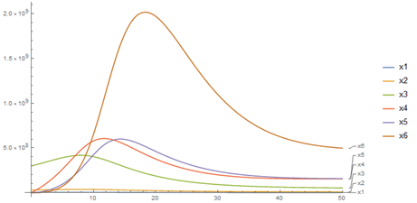
Figure 1 Case of six compartments for a 1 =0.7, a 2 =0.65, a 3 =0.65, a 4 =0.65, a 5 =0.55, p 1 =0.8, p 2 =0.11, p 3 =0.17, p 4 =0.34, p 5 =0.69,μ=0.3conk=1,2 10 9 MathType@MTEF@5@5@+= feaagKart1ev2aaatCvAUfeBSjuyZL2yd9gzLbvyNv2CaerbuLwBLn hiov2DGi1BTfMBaeXatLxBI9gBaerbd9wDYLwzYbItLDharqqtubsr 4rNCHbGeaGqkY=Mj0xXdbba91rFfpec8Eeeu0xXdbba9frFj0=OqFf ea0dXdd9vqaq=JfrVkFHe9pgea0dXdar=Jb9hs0dXdbPYxe9vr0=vr 0=vqpWqaaeaabiGaciaacaqabeaadaqaaqaaaOqaaiaadggadaWgaa WcbaGaaGymaaqabaGccqGH9aqpcaaIWaGaaiOlaiaaiEdacaGGSaGa amyyamaaBaaaleaacaaIYaaabeaakiabg2da9iaaicdacaGGUaGaaG OnaiaaiwdacaGGSaGaamyyamaaBaaaleaacaaIZaaabeaakiabg2da 9iaaicdacaGGUaGaaGOnaiaaiwdacaGGSaGaamyyamaaBaaaleaaca aI0aaabeaakiabg2da9iaaicdacaGGUaGaaGOnaiaaiwdacaGGSaGa amyyamaaBaaaleaacaaI1aaabeaakiabg2da9iaaicdacaGGUaGaaG ynaiaaiwdacaGGSaGaamiCamaaBaaaleaacaaIXaaabeaakiabg2da 9iaaicdacaGGUaGaaGioaiaacYcacaWGWbWaaSbaaSqaaiaaikdaae qaaOGaeyypa0JaaGimaiaac6cacaaIXaGaaGymaiaacYcacaWGWbWa aSbaaSqaaiaaiodaaeqaaOGaeyypa0JaaGimaiaac6cacaaIXaGaaG 4naiaacYcacaWGWbWaaSbaaSqaaiaaisdaaeqaaOGaeyypa0JaaGim aiaac6cacaaIZaGaaGinaiaacYcacaWGWbWaaSbaaSqaaiaaiwdaae qaaOGaeyypa0JaaGimaiaac6cacaaI2aGaaGyoaiaacYcacqaH8oqB cqGH9aqpcaaIWaGaaiOlaiaaiodacaWGJbGaam4Baiaad6gacaWGRb Gaeyypa0JaaGymaiaacYcacaaIYaGaey4fIOIaaGymaiaaicdadaah aaWcbeqaaiabgkHiTiaaiMdaaaaaaa@86A7@ , c 1 ( 0 )= 10 5 , c 2 ( 0 )= 10 6 , c 3 ( 0 )= 10 7 , c 4 ( 0 )=0, c 5 ( 0 )=0, c 6 ( 0 )=0 MathType@MTEF@5@5@+= feaagKart1ev2aaatCvAUfeBSjuyZL2yd9gzLbvyNv2CaerbuLwBLn hiov2DGi1BTfMBaeXatLxBI9gBaerbd9wDYLwzYbItLDharqqtubsr 4rNCHbGeaGqkY=Mj0xXdbba91rFfpec8Eeeu0xXdbba9frFj0=OqFf ea0dXdd9vqaq=JfrVkFHe9pgea0dXdar=Jb9hs0dXdbPYxe9vr0=vr 0=vqpWqaaeaabiGaciaacaqabeaadaqaaqaaaOqaaiaadogadaWgaa WcbaGaaGymaaqabaGcdaqadaqaaiaaicdaaiaawIcacaGLPaaacqGH 9aqpcaaIXaGaaGimamaaCaaaleqabaGaaGynaaaakiaacYcacaWGJb WaaSbaaSqaaiaaikdaaeqaaOWaaeWaaeaacaaIWaaacaGLOaGaayzk aaGaeyypa0JaaGymaiaaicdadaahaaWcbeqaaiaaiAdaaaGccaGGSa Gaam4yamaaBaaaleaacaaIZaaabeaakmaabmaabaGaaGimaaGaayjk aiaawMcaaiabg2da9iaaigdacaaIWaWaaWbaaSqabeaacaaI3aaaaO GaaiilaiaadogadaWgaaWcbaGaaGinaaqabaGcdaqadaqaaiaaicda aiaawIcacaGLPaaacqGH9aqpcaaIWaGaaiilaiaadogadaWgaaWcba GaaGynaaqabaGcdaqadaqaaiaaicdaaiaawIcacaGLPaaacqGH9aqp caaIWaGaaiilaiaadogadaWgaaWcbaGaaGOnaaqabaGcdaqadaqaai aaicdaaiaawIcacaGLPaaacqGH9aqpcaaIWaaaaa@62CB@ and final time t = 50.

The parameters and initial conditions were taken from Pa´zdziorek Pl.16 In the deterministic model, an accelerated increase in the population of mature cells in the final stage is obtained during days 10 and 20, and between days 20 and 40 this number decreases, remaining stable for more than 40 days. Clinical data report an average recovery when the patient has more than 1.5 * 10 ^ 8 mature cells per liter of body blood, this system offers us an ideal vision of the result that may be in contrast to the actual data.

The stochastic model

We now present a stochastic version of the deterministic model (2). The last deterministic number of differential equations is transformed into a system of stochastic differential equations as follows:

d ξ 1 =( ( 2 a 1 1+k ξ n (t) 1) ) p 1 ξ 1 (t) μ 1 ξ 1 (t) )dt+ α 1 ξ 1 (t)d W 1,t d ξ 2 =( ( 2 a 1 1+k ξ n (t) 1) ) p 2 ξ 2 (t)+2(1 a 1 1+k ξ n (t) ) μ 1 ξ 1 (t) )dt+ α 1 ξ 1 (t)d W 1,t d ξ n =( 2(1 a n 1 1+k ξ n (t) ) p n 1 ξ n 1 (t) μ n ξ n (t) )dt+ α n ξ n (t)d W n,t MathType@MTEF@5@5@+= feaagKart1ev2aaatCvAUfeBSjuyZL2yd9gzLbvyNv2CaerbuLwBLn hiov2DGi1BTfMBaeXatLxBI9gBaerbd9wDYLwzYbItLDharqqtubsr 4rNCHbGeaGqkY=Mj0xXdbba91rFfpec8Eeeu0xXdbba9frFj0=OqFf ea0dXdd9vqaq=JfrVkFHe9pgea0dXdar=Jb9hs0dXdbPYxe9vr0=vr 0=vqpWqaaeaabiGaciaacaqabeaadaqaaqaaaOabaeqabaqcLbsaca WGKbGaeqOVdGNcdaWgaaWcbaGaaGymaaqabaqcLbsacqGH9aqpkmaa bmaabaWaaeWaaeaadaWcaaqaaKqzGeGaaGOmaiaadggakmaaBaaale aacaaIXaaabeaaaOqaaKqzGeGaaGymaiabgUcaRiaadUgacqaH+oaE kmaaBaaaleaacaWGUbaabeaajugibiaacIcacaWG0bGaaiykaaaacq GHsislcaaIXaGaaiykaaGccaGLOaGaayzkaaqcLbsacaaMc8UaaGPa VlaadchakmaaBaaaleaacaaIXaaabeaajugibiabe67a4PWaaSbaaS qaaiaaigdaaeqaaKqzGeGaaiikaiaadshacaGGPaGaeyOeI0IaeqiV d0McdaWgaaWcbaGaaGymaaqabaqcLbsacqaH+oaEkmaaBaaaleaaca aIXaaabeaajugibiaacIcacaWG0bGaaiykaaGccaGLOaGaayzkaaqc LbsacaaMc8UaamizaiaadshacqGHRaWkcqaHXoqykmaaBaaaleaaca aIXaaabeaajugibiabe67a4PWaaSbaaSqaaiaaigdaaeqaaKqzGeGa aiikaiaadshacaGGPaGaamizaiaadEfakmaaBaaaleaacaaIXaGaai ilaiaadshaaeqaaaGcbaqcLbsacaWGKbGaeqOVdGNcdaWgaaWcbaGa aGOmaaqabaGccqGH9aqpdaqadaqaamaabmaabaWaaSaaaeaajugibi aaikdacaWGHbGcdaWgaaWcbaGaaGymaaqabaaakeaajugibiaaigda cqGHRaWkcaWGRbGaeqOVdGNcdaWgaaWcbaGaamOBaaqabaqcLbsaca GGOaGaamiDaiaacMcaaaGaeyOeI0IaaGymaiaacMcaaOGaayjkaiaa wMcaaKqzGeGaaGPaVlaaykW7caWGWbGcdaWgaaWcbaGaaGOmaaqaba qcLbsacqaH+oaEkmaaBaaaleaacaaIYaaabeaajugibiaacIcacaWG 0bGaaiykaiabgUcaRiaaikdacaGGOaGaaGymaiabgkHiTOWaaSaaae aajugibiaadggakmaaBaaaleaacaaIXaaabeaaaOqaaKqzGeGaaGym aiabgUcaRiaadUgacqaH+oaEkmaaBaaaleaacaWGUbaabeaajugibi aacIcacaWG0bGaaiykaaaakiaacMcacqGHsisljugibiabeY7aTPWa aSbaaSqaaiaaigdaaeqaaKqzGeGaeqOVdGNcdaWgaaWcbaGaaGymaa qabaqcLbsacaGGOaGaamiDaiaacMcaaOGaayjkaiaawMcaaKqzGeGa aGPaVlaadsgacaWG0bGaey4kaSIaeqySdeMcdaWgaaWcbaGaaGymaa qabaqcLbsacqaH+oaEkmaaBaaaleaacaaIXaaabeaajugibiaacIca caWG0bGaaiykaiaadsgacaWGxbGcdaWgaaWcbaGaaGymaiaacYcaca WG0baabeaaaOqaaKqzGeGaamizaiabe67a4PWaaSbaaSqaaiaad6ga aeqaaOGaeyypa0ZaaeWaaeaacaaIYaGaaiikaiaaigdacqGHsislda WcaaqaaKqzGeGaamyyaOWaaSbaaSqaaiaad6gacqGHsislaeqaaOWa aSbaaSqaaiaaigdaaeqaaaGcbaqcLbsacaaIXaGaey4kaSIaam4Aai abe67a4PWaaSbaaSqaaiaad6gaaeqaaKqzGeGaaiikaiaadshacaGG PaaaaOGaaiykaiaacchadaWgaaWcbaWaaSbaaWqaaiaad6gacqGHsi slaeqaaaWcbeaakmaaBaaaleaakmaaBaaaleaajugibiaaigdaaSqa baqcLbsacqaH+oaEkmaaBaaaleaakmaaBaaameaajugibiaad6gaaW qabaqcLbsacqGHsislcaaIXaaaleqaaKqzGeGaaiikaiaadshacaGG PaGaeyOeI0caleqaaKqzGeGaeqiVd0McdaWgaaWcbaGaamOBaaqaba qcLbsacqaH+oaEkmaaBaaaleaacaWGUbaabeaajugibiaacIcacaWG 0bGccaGGPaaacaGLOaGaayzkaaGaamizaiaadshacqGHRaWkjugibi abeg7aHPWaaSbaaSqaaiaad6gaaeqaaKqzGeGaeqOVdGNcdaWgaaWc baGaamOBaaqabaqcLbsacaGGOaGaamiDaiaacMcacaWGKbGaam4vaO WaaSbaaSqaaiaad6gacaGGSaGaaiiDaaqabaaaaaa@0754@   (6)

Where the stochastic processes ξ 1 , ξ 2 ,.........., ξ n MathType@MTEF@5@5@+= feaagKart1ev2aaatCvAUfeBSjuyZL2yd9gzLbvyNv2CaerbuLwBLn hiov2DGi1BTfMBaeXatLxBI9gBaerbd9wDYLwzYbItLDharqqtubsr 4rNCHbGeaGqkY=Mj0xXdbba91rFfpec8Eeeu0xXdbba9frFj0=OqFf ea0dXdd9vqaq=JfrVkFHe9pgea0dXdar=Jb9hs0dXdbPYxe9vr0=vr 0=vqpWqaaeaabiGaciaacaqabeaadaqaaqaaaOqaaiabe67a4naaBa aaleaacaaIXaaabeaakiaacYcacqaH+oaEdaWgaaWcbaGaaGOmaaqa baGccaGGSaGaaiOlaiaac6cacaGGUaGaaiOlaiaac6cacaGGUaGaai Olaiaac6cacaGGUaGaaiOlaiaacYcacqaH+oaEdaWgaaWcbaGaamOB aaqabaaaaa@485D@  describe the densities of the population of stem cells, cells at different stages of differentiation and mature cells. The coefficients a i , p i MathType@MTEF@5@5@+= feaagKart1ev2aaatCvAUfeBSjuyZL2yd9gzLbvyNv2CaerbuLwBLn hiov2DGi1BTfMBaeXatLxBI9gBaerbd9wDYLwzYbItLDharqqtubsr 4rNCHbGeaGqkY=Mj0xXdbba91rFfpec8Eeeu0xXdbba9frFj0=OqFf ea0dXdd9vqaq=JfrVkFHe9pgea0dXdar=Jb9hs0dXdbPYxe9vr0=vr 0=vqpWqaaeaabiGaciaacaqabeaadaqaaqaaaOqaaiaadggadaWgaa WcbaGaamyAaaqabaGccaGGSaGaamiCamaaBaaaleaacaWGPbaabeaa aaa@3BD7@  for i=1,...,n1 MathType@MTEF@5@5@+= feaagKart1ev2aaatCvAUfeBSjuyZL2yd9gzLbvyNv2CaerbuLwBLn hiov2DGi1BTfMBaeXatLxBI9gBaerbd9wDYLwzYbItLDharqqtubsr 4rNCHbGeaGqkY=Mj0xXdbba91rFfpec8Eeeu0xXdbba9frFj0=OqFf ea0dXdd9vqaq=JfrVkFHe9pgea0dXdar=Jb9hs0dXdbPYxe9vr0=vr 0=vqpWqaaeaabiGaciaacaqabeaadaqaaqaaaOqaaiaadMgacqGH9a qpcaaIXaGaaiilaiaac6cacaGGUaGaaiOlaiaacYcacaWGUbGaeyOe I0IaaGymaaaa@3FCE@  and μ i MathType@MTEF@5@5@+= feaagKart1ev2aaatCvAUfeBSjuyZL2yd9gzLbvyNv2CaerbuLwBLn hiov2DGi1BTfMBaeXatLxBI9gBaerbd9wDYLwzYbItLDharqqtubsr 4rNCHbGeaGqkY=Mj0xXdbba91rFfpec8Eeeu0xXdbba9frFj0=OqFf ea0dXdd9vqaq=JfrVkFHe9pgea0dXdar=Jb9hs0dXdbPYxe9vr0=vr 0=vqpWqaaeaabiGaciaacaqabeaadaqaaqaaaOqaaiabeY7aTnaaBa aaleaacaWGPbaabeaaaaa@39DE@  for i=1,...,n MathType@MTEF@5@5@+= feaagKart1ev2aaatCvAUfeBSjuyZL2yd9gzLbvyNv2CaerbuLwBLn hiov2DGi1BTfMBaeXatLxBI9gBaerbd9wDYLwzYbItLDharqqtubsr 4rNCHbGeaGqkY=Mj0xXdbba91rFfpec8Eeeu0xXdbba9frFj0=OqFf ea0dXdd9vqaq=JfrVkFHe9pgea0dXdar=Jb9hs0dXdbPYxe9vr0=vr 0=vqpWqaaeaabiGaciaacaqabeaadaqaaqaaaOqaaiaadMgacqGH9a qpcaaIXaGaaiilaiaac6cacaGGUaGaaiOlaiaacYcacaWGUbaaaa@3E26@  satisfy the assumptions (3), (4). ( W 1,t ,... W n,t ) MathType@MTEF@5@5@+= feaagKart1ev2aaatCvAUfeBSjuyZL2yd9gzLbvyNv2CaerbuLwBLn hiov2DGi1BTfMBaeXatLxBI9gBaerbd9wDYLwzYbItLDharqqtubsr 4rNCHbGeaGqkY=Mj0xXdbba91rFfpec8Eeeu0xXdbba9frFj0=OqFf ea0dXdd9vqaq=JfrVkFHe9pgea0dXdar=Jb9hs0dXdbPYxe9vr0=vr 0=vqpWqaaeaabiGaciaacaqabeaadaqaaqaaaOqaamaabmaabaGaam 4vamaaBaaaleaacaaIXaGaaiilaiaadshaaeqaaOGaaiilaiaac6ca caGGUaGaaiOlaiaadEfadaWgaaWcbaGaaiOBaiaacYcacaWG0baabe aaaOGaayjkaiaawMcaaaaa@4280@  is a n-dimensional Wiener process and α i MathType@MTEF@5@5@+= feaagKart1ev2aaatCvAUfeBSjuyZL2yd9gzLbvyNv2CaerbuLwBLn hiov2DGi1BTfMBaeXatLxBI9gBaerbd9wDYLwzYbItLDharqqtubsr 4rNCHbGeaGqkY=Mj0xXdbba91rFfpec8Eeeu0xXdbba9frFj0=OqFf ea0dXdd9vqaq=JfrVkFHe9pgea0dXdar=Jb9hs0dXdbPYxe9vr0=vr 0=vqpWqaaeaabiGaciaacaqabeaadaqaaqaaaOqaaiabeg7aHnaaBa aaleaacaWGPbaabeaaaaa@39C7@  for i=1,...,n MathType@MTEF@5@5@+= feaagKart1ev2aaatCvAUfeBSjuyZL2yd9gzLbvyNv2CaerbuLwBLn hiov2DGi1BTfMBaeXatLxBI9gBaerbd9wDYLwzYbItLDharqqtubsr 4rNCHbGeaGqkY=Mj0xXdbba91rFfpec8Eeeu0xXdbba9frFj0=OqFf ea0dXdd9vqaq=JfrVkFHe9pgea0dXdar=Jb9hs0dXdbPYxe9vr0=vr 0=vqpWqaaeaabiGaciaacaqabeaadaqaaqaaaOqaaiaadMgacqGH9a qpcaaIXaGaaiilaiaac6cacaGGUaGaaiOlaiaacYcacaWGUbaaaa@3E26@  are positive.

Mathematical and biological justification of the stochastic system

This section shows the six-dimensional version (compartments) of the stochastic model of the stochastic system. For this, the noise term is maintained in each compartment and the population densities are treated as stochastic processes. The noise term is made up of the population density of the cell type of the indicated compartment, the Wiener process, independent of the rest of the processes and an α>0 MathType@MTEF@5@5@+= feaagKart1ev2aaatCvAUfeBSjuyZL2yd9gzLbvyNv2CaerbuLwBLn hiov2DGi1BTfMBaeXatLxBI9gBaerbd9wDYLwzYbItLDharqqtubsr 4rNCHbGeaGqkY=Mj0xXdbba91rFfpec8Eeeu0xXdbba9frFj0=OqFf ea0dXdd9vqaq=JfrVkFHe9pgea0dXdar=Jb9hs0dXdbPYxe9vr0=vr 0=vqpWqaaeaabiGaciaacaqabeaadaqaaqaaaOqaaiabeg7aHjabg6 da+iaaicdaaaa@3A6F@ , which regulates the intensity of the Wiener process in each equation. That equations represent the population dynamics of the cells in the different stages of maturation. So that the smaller the system is closer to the deterministic model and as it increases, the greater the Wiener process has in the solution that is gets.

 The deterministic model is developed in an ideal environment, without influence of the external environment for the rates of self-renewal and proliferation. For the development of this investigation the term of noise is added. It is desired to reach conclusions on the influence of the environment during the process of cell division and maturation, applying different levels of stochastic noise intensity in each compartment. The process of cell division and maturation is represented as a Markov chain. So, it is necessary to use an independent Wiener process at each stage, since the population density of each compartment i at time t only depends on its own density in that same instant of time. In addition, the Wiener process is used because the model on cell division is raised from in vitro culture or in some type of fluid, which represents a Brownian movement with statistically independent and stationary increases.

In biological terms, this fluid produces different random stimuli, which together with the different feedback signals on the stem cells at each stage of the culture, can influence the speed of realization of the process of cell division and maturation and the density and quantity of cells, both of the first type (stem cells), and of the required final result (mature cells), at the end of the culture time in the applied environment.

6-dimensional model (hematopoietic cell)

The following section shows the six-compartment version of the general model on cell maturation presented in the previous section, which represents the cell cycle for hematopoietic stem cells. This is solved using the parameters used in the deterministic model proposed in9 with randomly selected noise levels, which include low and high levels compared to the models previously analyzed, because the intensity of the same can have different effects when vary the number of dimensions analyzed in the stochastic system. The model proposed for six dimensions is as follows:

d ξ 1 [ t ]=( ( 2 a 1 1+k ξ 6 [ t ] ) p 1 ξ 1 [ t ] )dt+ α 1 ξ 1 [ t ]d w 1 [ t ] d ξ 2 [ t ]=( ( 2 a 2 1+k ξ 6 [ t ] 1 ) p 2 ξ 2 [ t ]+2( 1 a 1 1+k ξ 6 [ t ] ) p 1 ξ 1 [ t ] )dt+ α 2 ξ 2 [ t ]d w 2 [ t ] d ξ 3 [ t ]=( ( 2 a 3 1+k ξ 6 [ t ] 1 ) p 3 ξ 3 [ t ]+2( 1 a 2 1+k ξ 6 [ t ] ) p 2 ξ 2 [ t ] )dt+ α 3 ξ 3 [ t ]d w 3 [ t ] d ξ 4 [ t ]=( ( 2 a 4 1+k ξ 6 [ t ] 1 ) p 4 ξ 4 [ t ]+2( 1 a 3 1+k ξ 6 [ t ] ) p 3 ξ 3 [ t ] )dt+ α 4 ξ 4 [ t ]d w 4 [ t ] d ξ 5 [ t ]=( ( 2 a 5 1+k ξ 6 [ t ] 1 ) p 5 ξ 5 [ t ]+2( 1 a 4 1+k ξ 6 [ t ] ) p 4 ξ 4 [ t ] )dt+ α 5 ξ 5 [ t ]d w 5 [ t ] d ξ 6 [ t ]=( 2( 1 a 5 1+k ξ 6 [ t ] ) p 5 ξ 5 [ t ]μ ξ 6 [ t ] )dt+ α 6 ξ 6 [ t ]d w 6 [ t ] MathType@MTEF@5@5@+= feaagKart1ev2aaatCvAUfeBSjuyZL2yd9gzLbvyNv2CaerbuLwBLn hiov2DGi1BTfMBaeXatLxBI9gBaerbd9wDYLwzYbItLDharqqtubsr 4rNCHbGeaGqkY=Mj0xXdbba91rFfpec8Eeeu0xXdbba9frFj0=OqFf ea0dXdd9vqaq=JfrVkFHe9pgea0dXdar=Jb9hs0dXdbPYxe9vr0=vr 0=vqpWqaaeaabiGaciaacaqabeaadaqaaqaaaOabaeqabaGaamizai abe67a4naaBaaaleaacaaIXaaabeaakmaadmaabaGaamiDaaGaay5w aiaaw2faaiabg2da9maabmaabaWaaeWaaeaadaWcaaqaaiaaikdaca WGHbWaaSbaaSqaaiaaigdaaeqaaaGcbaGaaGymaiabgUcaRiaadUga cqaH+oaEdaWgaaWcbaGaaGOnaaqabaGcdaWadaqaaiaadshaaiaawU facaGLDbaaaaaacaGLOaGaayzkaaGaamiCamaaBaaaleaacaaIXaaa beaakiabe67a4naaBaaaleaacaaIXaaabeaakmaadmaabaGaamiDaa Gaay5waiaaw2faaaGaayjkaiaawMcaaiaadsgacaWG0bGaey4kaSIa eqySde2aaSbaaSqaaiaaigdaaeqaaOGaeqOVdG3aaSbaaSqaaiaaig daaeqaaOWaamWaaeaacaWG0baacaGLBbGaayzxaaGaamizaiaadEha daWgaaWcbaGaaGymaaqabaGcdaWadaqaaiaadshaaiaawUfacaGLDb aaaeaacaWGKbGaeqOVdG3aaSbaaSqaaiaaikdaaeqaaOWaamWaaeaa caWG0baacaGLBbGaayzxaaGaeyypa0ZaaeWaaeaadaqadaqaamaala aabaGaaGOmaiaadggadaWgaaWcbaGaaGOmaaqabaaakeaacaaIXaGa ey4kaSIaam4Aaiabe67a4naaBaaaleaacaaI2aaabeaakmaadmaaba GaamiDaaGaay5waiaaw2faaaaacqGHsislcaaIXaaacaGLOaGaayzk aaGaamiCamaaBaaaleaacaaIYaaabeaakiabe67a4naaBaaaleaaca aIYaaabeaakmaadmaabaGaamiDaaGaay5waiaaw2faaiabgUcaRiaa ikdadaqadaqaaiaaigdacqGHsisldaWcaaqaaiaadggadaWgaaWcba GaaGymaaqabaaakeaacaaIXaGaey4kaSIaam4AaiabgEHiQiabe67a 4naaBaaaleaacaaI2aaabeaakmaadmaabaGaamiDaaGaay5waiaaw2 faaaaaaiaawIcacaGLPaaacaWGWbWaaSbaaSqaaiaaigdaaeqaaOGa eqOVdG3aaSbaaSqaaiaaigdaaeqaaOWaamWaaeaacaWG0baacaGLBb GaayzxaaaacaGLOaGaayzkaaGaamizaiaadshacqGHRaWkcqaHXoqy daWgaaWcbaGaaGOmaaqabaGccqaH+oaEdaWgaaWcbaGaaGOmaaqaba GcdaWadaqaaiaadshaaiaawUfacaGLDbaacaWGKbGaam4DamaaBaaa leaacaaIYaaabeaakmaadmaabaGaamiDaaGaay5waiaaw2faaaqaai aadsgacqaH+oaEdaWgaaWcbaGaaG4maaqabaGcdaWadaqaaiaadsha aiaawUfacaGLDbaacqGH9aqpdaqadaqaamaabmaabaWaaSaaaeaaca aIYaGaamyyamaaBaaaleaacaaIZaaabeaaaOqaaiaaigdacqGHRaWk caWGRbGaeqOVdG3aaSbaaSqaaiaaiAdaaeqaaOWaamWaaeaacaWG0b aacaGLBbGaayzxaaaaaiabgkHiTiaaigdaaiaawIcacaGLPaaacaWG WbWaaSbaaSqaaiaaiodaaeqaaOGaeqOVdG3aaSbaaSqaaiaaiodaae qaaOWaamWaaeaacaWG0baacaGLBbGaayzxaaGaey4kaSIaaGOmamaa bmaabaGaaGymaiabgkHiTmaalaaabaGaamyyamaaBaaaleaacaaIYa aabeaaaOqaaiaaigdacqGHRaWkcaWGRbGaey4fIOIaeqOVdG3aaSba aSqaaiaaiAdaaeqaaOWaamWaaeaacaWG0baacaGLBbGaayzxaaaaaa GaayjkaiaawMcaaiaadchadaWgaaWcbaGaaGOmaaqabaGccqaH+oaE daWgaaWcbaGaaGOmaaqabaGcdaWadaqaaiaadshaaiaawUfacaGLDb aaaiaawIcacaGLPaaacaWGKbGaamiDaiabgUcaRiabeg7aHnaaBaaa leaacaaIZaaabeaakiabe67a4naaBaaaleaacaaIZaaabeaakmaadm aabaGaamiDaaGaay5waiaaw2faaiaadsgacaWG3bWaaSbaaSqaaiaa iodaaeqaaOWaamWaaeaacaWG0baacaGLBbGaayzxaaaabaGaamizai abe67a4naaBaaaleaacaaI0aaabeaakmaadmaabaGaamiDaaGaay5w aiaaw2faaiabg2da9maabmaabaWaaeWaaeaadaWcaaqaaiaaikdaca WGHbWaaSbaaSqaaiaaisdaaeqaaaGcbaGaaGymaiabgUcaRiaadUga cqaH+oaEdaWgaaWcbaGaaGOnaaqabaGcdaWadaqaaiaadshaaiaawU facaGLDbaaaaGaeyOeI0IaaGymaaGaayjkaiaawMcaaiaadchadaWg aaWcbaGaaGinaaqabaGccqaH+oaEdaWgaaWcbaGaaGinaaqabaGcda WadaqaaiaadshaaiaawUfacaGLDbaacqGHRaWkcaaIYaWaaeWaaeaa caaIXaGaeyOeI0YaaSaaaeaacaWGHbWaaSbaaSqaaiaaiodaaeqaaa GcbaGaaGymaiabgUcaRiaadUgacqGHxiIkcqaH+oaEdaWgaaWcbaGa aGOnaaqabaGcdaWadaqaaiaadshaaiaawUfacaGLDbaaaaaacaGLOa GaayzkaaGaamiCamaaBaaaleaacaaIZaaabeaakiabe67a4naaBaaa leaacaaIZaaabeaakmaadmaabaGaamiDaaGaay5waiaaw2faaaGaay jkaiaawMcaaiaadsgacaWG0bGaey4kaSIaeqySde2aaSbaaSqaaiaa isdaaeqaaOGaeqOVdG3aaSbaaSqaaiaaisdaaeqaaOWaamWaaeaaca WG0baacaGLBbGaayzxaaGaamizaiaadEhadaWgaaWcbaGaaGinaaqa baGcdaWadaqaaiaadshaaiaawUfacaGLDbaaaeaacaWGKbGaeqOVdG 3aaSbaaSqaaiaaiwdaaeqaaOWaamWaaeaacaWG0baacaGLBbGaayzx aaGaeyypa0ZaaeWaaeaadaqadaqaamaalaaabaGaaGOmaiaadggada WgaaWcbaGaaGynaaqabaaakeaacaaIXaGaey4kaSIaam4Aaiabe67a 4naaBaaaleaacaaI2aaabeaakmaadmaabaGaamiDaaGaay5waiaaw2 faaaaacqGHsislcaaIXaaacaGLOaGaayzkaaGaamiCamaaBaaaleaa caaI1aaabeaakiabe67a4naaBaaaleaacaaI1aaabeaakmaadmaaba GaamiDaaGaay5waiaaw2faaiabgUcaRiaaikdadaqadaqaaiaaigda cqGHsisldaWcaaqaaiaadggadaWgaaWcbaGaaGinaaqabaaakeaaca aIXaGaey4kaSIaam4AaiabgEHiQiabe67a4naaBaaaleaacaaI2aaa beaakmaadmaabaGaamiDaaGaay5waiaaw2faaaaaaiaawIcacaGLPa aacaWGWbWaaSbaaSqaaiaaisdaaeqaaOGaeqOVdG3aaSbaaSqaaiaa isdaaeqaaOWaamWaaeaacaWG0baacaGLBbGaayzxaaaacaGLOaGaay zkaaGaamizaiaadshacqGHRaWkcqaHXoqydaWgaaWcbaGaaGynaaqa baGccqaH+oaEdaWgaaWcbaGaaGynaaqabaGcdaWadaqaaiaadshaai aawUfacaGLDbaacaWGKbGaam4DamaaBaaaleaacaaI1aaabeaakmaa dmaabaGaamiDaaGaay5waiaaw2faaaqaaiaadsgacqaH+oaEdaWgaa WcbaGaaGOnaaqabaGcdaWadaqaaiaadshaaiaawUfacaGLDbaacqGH 9aqpdaqadaqaaiaaikdadaqadaqaaiaaigdacqGHsisldaWcaaqaai aadggadaWgaaWcbaGaaGynaaqabaaakeaacaaIXaGaey4kaSIaam4A aiabgEHiQiabe67a4naaBaaaleaacaaI2aaabeaakmaadmaabaGaam iDaaGaay5waiaaw2faaaaaaiaawIcacaGLPaaacaWGWbWaaSbaaSqa aiaaiwdaaeqaaOGaeqOVdG3aaSbaaSqaaiaaiwdaaeqaaOWaamWaae aacaWG0baacaGLBbGaayzxaaGaeyOeI0IaeqiVd0MaeqOVdG3aaSba aSqaaiaaiAdaaeqaaOWaamWaaeaacaWG0baacaGLBbGaayzxaaaaca GLOaGaayzkaaGaamizaiaadshacqGHRaWkcqaHXoqydaWgaaWcbaGa aGOnaaqabaGccqaH+oaEdaWgaaWcbaGaaGOnaaqabaGcdaWadaqaai aadshaaiaawUfacaGLDbaacaWGKbGaam4DamaaBaaaleaacaaI2aaa beaakmaadmaabaGaamiDaaGaay5waiaaw2faaaaaaa@B889@   (12)

Evaluated for a 1 =0.51, a 2 = a 3 = a 4 =0.475, a 5 =0.41 MathType@MTEF@5@5@+= feaagKart1ev2aaatCvAUfeBSjuyZL2yd9gzLbvyNv2CaerbuLwBLn hiov2DGi1BTfMBaeXatLxBI9gBaerbd9wDYLwzYbItLDharqqtubsr 4rNCHbGeaGqkY=Mj0xXdbba91rFfpec8Eeeu0xXdbba9frFj0=OqFf ea0dXdd9vqaq=JfrVkFHe9pgea0dXdar=Jb9hs0dXdbPYxe9vr0=vr 0=vqpWqaaeaabiGaciaacaqabeaadaqaaqaaaOqaaiaadggadaWgaa WcbaGaaGymaaqabaGccqGH9aqpcaaIWaGaaiOlaiaaiwdacaaIXaGa aiilaiaadggadaWgaaWcbaGaaGOmaaqabaGccqGH9aqpcaWGHbWaaS baaSqaaiaaiodaaeqaaOGaeyypa0JaamyyamaaBaaaleaacaaI0aaa beaakiabg2da9iaaicdacaGGUaGaaGinaiaaiEdacaaI1aGaaiilai aadggadaWgaaWcbaGaaGynaaqabaGccqGH9aqpcaaIWaGaaiOlaiaa isdacaaIXaaaaa@503E@ , p 1 =0.173, p 2 =0.231, p 3 =0.347, p 4 =0.693, p 5 =1.386 MathType@MTEF@5@5@+= feaagKart1ev2aaatCvAUfeBSjuyZL2yd9gzLbvyNv2CaerbuLwBLn hiov2DGi1BTfMBaeXatLxBI9gBaerbd9wDYLwzYbItLDharqqtubsr 4rNCHbGeaGqkY=Mj0xXdbba91rFfpec8Eeeu0xXdbba9frFj0=OqFf ea0dXdd9vqaq=JfrVkFHe9pgea0dXdar=Jb9hs0dXdbPYxe9vr0=vr 0=vqpWqaaeaabiGaciaacaqabeaadaqaaqaaaOqaaiaadchadaWgaa WcbaGaaGymaaqabaGccqGH9aqpcaaIWaGaaiOlaiaaigdacaaI3aGa aG4maiaacYcacaWGWbWaaSbaaSqaaiaaikdaaeqaaOGaeyypa0JaaG imaiaac6cacaaIYaGaaG4maiaaigdacaGGSaGaamiCamaaBaaaleaa caaIZaaabeaakiabg2da9iaaicdacaGGUaGaaG4maiaaisdacaaI3a GaaiilaiaadchadaWgaaWcbaGaaGinaaqabaGccqGH9aqpcaaIWaGa aiOlaiaaiAdacaaI5aGaaG4maiaacYcacaWGWbWaaSbaaSqaaiaaiw daaeqaaOGaeyypa0JaaGymaiaac6cacaaIZaGaaGioaiaaiAdaaaa@5AB9@ , μ=0.3,k=1.28 10 9 MathType@MTEF@5@5@+= feaagKart1ev2aaatCvAUfeBSjuyZL2yd9gzLbvyNv2CaerbuLwBLn hiov2DGi1BTfMBaeXatLxBI9gBaerbd9wDYLwzYbItLDharqqtubsr 4rNCHbGeaGqkY=Mj0xXdbba91rFfpec8Eeeu0xXdbba9frFj0=OqFf ea0dXdd9vqaq=JfrVkFHe9pgea0dXdar=Jb9hs0dXdbPYxe9vr0=vr 0=vqpWqaaeaabiGaciaacaqabeaadaqaaqaaaOqaaiabeY7aTjabg2 da9iaaicdacaGGUaGaaG4maiaacYcacaWGRbGaeyypa0JaaGymaiaa c6cacaaIYaGaaGioaiabgEHiQiaaigdacaaIWaWaaWbaaSqabeaacq GHsislcaaI5aaaaaaa@45C5@  and initials conditions ξ 1 ( 0 )= 10 5 , ξ 2 ( 0 )= 10 6 , ξ 3 ( 0 )= 10 9 , ξ 4 = ξ 5 = ξ 6 =0 MathType@MTEF@5@5@+= feaagKart1ev2aaatCvAUfeBSjuyZL2yd9gzLbvyNv2CaerbuLwBLn hiov2DGi1BTfMBaeXatLxBI9gBaerbd9wDYLwzYbItLDharqqtubsr 4rNCHbGeaGqkY=Mj0xXdbba91rFfpec8Eeeu0xXdbba9frFj0=OqFf ea0dXdd9vqaq=JfrVkFHe9pgea0dXdar=Jb9hs0dXdbPYxe9vr0=vr 0=vqpWqaaeaabiGaciaacaqabeaadaqaaqaaaOqaaiabe67a4naaBa aaleaacaaIXaaabeaakmaabmaabaGaaGimaaGaayjkaiaawMcaaiab g2da9iaaigdacaaIWaWaaWbaaSqabeaacaaI1aaaaOGaaiilaiabe6 7a4naaBaaaleaacaaIYaaabeaakmaabmaabaGaaGimaaGaayjkaiaa wMcaaiabg2da9iaaigdacaaIWaWaaWbaaSqabeaacaaI2aaaaOGaai ilaiabe67a4naaBaaaleaacaaIZaaabeaakmaabmaabaGaaGimaaGa ayjkaiaawMcaaiabg2da9iaaigdacaaIWaWaaWbaaSqabeaacaaI5a aaaOGaaiilaiabe67a4naaBaaaleaacaaI0aaabeaakiabg2da9iab e67a4naaBaaaleaacaaI1aaabeaakiabg2da9iabe67a4naaBaaale aacaaI2aaabeaakiabg2da9iaaicdaaaa@5E52@ , e noise intensities for α 1 =0.011, α 2 =0.013, α 3 =0.015, α 4 =0.017, α 5 =0.019, α 6 =0.025 MathType@MTEF@5@5@+= feaagKart1ev2aaatCvAUfeBSjuyZL2yd9gzLbvyNv2CaerbuLwBLn hiov2DGi1BTfMBaeXatLxBI9gBaerbd9wDYLwzYbItLDharqqtubsr 4rNCHbGeaGqkY=Mj0xXdbba91rFfpec8Eeeu0xXdbba9frFj0=OqFf ea0dXdd9vqaq=JfrVkFHe9pgea0dXdar=Jb9hs0dXdbPYxe9vr0=vr 0=vqpWqaaeaabiGaciaacaqabeaadaqaaqaaaOqaaiabeg7aHnaaBa aaleaacaaIXaaabeaakiabg2da9iaaicdacaGGUaGaaGimaiaaigda caaIXaGaaiilaiabeg7aHnaaBaaaleaacaaIYaaabeaakiabg2da9i aaicdacaGGUaGaaGimaiaaigdacaaIZaGaaiilaiabeg7aHnaaBaaa leaacaaIZaaabeaakiabg2da9iaaicdacaGGUaGaaGimaiaaigdaca aI1aGaaiilaiabeg7aHnaaBaaaleaacaaI0aaabeaakiabg2da9iaa icdacaGGUaGaaGimaiaaigdacaaI3aGaaiilaiabeg7aHnaaBaaale aacaaI1aaabeaakiabg2da9iaaicdacaGGUaGaaGimaiaaigdacaaI 5aGaaiilaiabeg7aHnaaBaaaleaacaaI2aaabeaakiabg2da9iaaic dacaGGUaGaaGimaiaaikdacaaI1aaaaa@65D2@

Using the Euler–Maruyama method, an approximation of the Gillespie Algorism whit the functions of ItoProcess and RandomFunction of Mathematica software, to resolves the system, then is as follows (Figure 2):
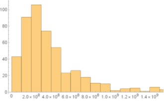
Figure 2 Histogram of 500 trajectories of the Six-dimensional model whit a t - final = 5 days, the same parameters to Figure 1.

The graph shows the results of 500 trajectories analyzing only the mature cell count using the stochastic SDE. For this, the same parameters are used as in the deterministic system and noise is added as a random real between 0 and 0.5 for each compartment during the 500 simulations. A simulation is performed with a final time of 50 days according to the final result of the deterministic model, where stability is reached. The implementation of this noise level is a little higher than what an average patient could present, so it is done by implementing the Gillespie Algorithm to give greater accuracy. It is observed how 91 trajectories are between 1.5 and 2.5 10 8 MathType@MTEF@5@5@+= feaagKart1ev2aaatCvAUfeBSjuyZL2yd9gzLbvyNv2CaerbuLwBLn hiov2DGi1BTfMBaeXatLxBI9gBaerbd9wDYLwzYbItLDharqqtubsr 4rNCHbGeaGqkY=Mj0xXdbba91rFfpec8Eeeu0xXdbba9frFj0=OqFf ea0dXdd9vqaq=JfrVkFHe9pgea0dXdar=Jb9hs0dXdbPYxe9vr0=vr 0=vqpWqaaeaabiGaciaacaqabeaadaqaaqaaaOqaaiaaikdacaGGUa GaaGynaiabgEHiQiaaigdacaaIWaWaaWbaaSqabeaacaaI4aaaaaaa @3C8E@ , 106 are between 2.5 and 3.5 10 8 MathType@MTEF@5@5@+= feaagKart1ev2aaatCvAUfeBSjuyZL2yd9gzLbvyNv2CaerbuLwBLn hiov2DGi1BTfMBaeXatLxBI9gBaerbd9wDYLwzYbItLDharqqtubsr 4rNCHbGeaGqkY=Mj0xXdbba91rFfpec8Eeeu0xXdbba9frFj0=OqFf ea0dXdd9vqaq=JfrVkFHe9pgea0dXdar=Jb9hs0dXdbPYxe9vr0=vr 0=vqpWqaaeaabiGaciaacaqabeaadaqaaqaaaOqaaiaaiodacaGGUa GaaGynaiabgEHiQiaaigdacaaIWaWaaWbaaSqabeaacaaI4aaaaaaa @3C8F@  and 74 between 3.5 and 4.5 10 8 MathType@MTEF@5@5@+= feaagKart1ev2aaatCvAUfeBSjuyZL2yd9gzLbvyNv2CaerbuLwBLn hiov2DGi1BTfMBaeXatLxBI9gBaerbd9wDYLwzYbItLDharqqtubsr 4rNCHbGeaGqkY=Mj0xXdbba91rFfpec8Eeeu0xXdbba9frFj0=OqFf ea0dXdd9vqaq=JfrVkFHe9pgea0dXdar=Jb9hs0dXdbPYxe9vr0=vr 0=vqpWqaaeaabiGaciaacaqabeaadaqaaqaaaOqaaiaaisdacaGGUa GaaGynaiabgEHiQiaaigdacaaIWaWaaWbaaSqabeaacaaI4aaaaaaa @3C90@  mature cells per liter of blood, coinciding with the clinical data taken from the bibliography and showing great accuracy due to the presence of the environmental noise factor during treatment. To verify that most of the trajectories are not null and are in the range obtained, the following representation was made (Figure 3):
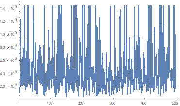
Figure 3 Represent the final results of the 500 trajectories employed in the solution of a stocastic model, using the leukocyte count on the y-axis and trajectory on the x-axis.

This graph shows the fluctuation of the final result of each trajectory, in which it is observable that practically none of them is null and are in the established range. A spontaneous approach is performed as a final verification resource that indicates how most of it focuses in the range of 2.0 to 4.0 10 8 MathType@MTEF@5@5@+= feaagKart1ev2aaatCvAUfeBSjuyZL2yd9gzLbvyNv2CaerbuLwBLn hiov2DGi1BTfMBaeXatLxBI9gBaerbd9wDYLwzYbItLDharqqtubsr 4rNCHbGeaGqkY=Mj0xXdbba91rFfpec8Eeeu0xXdbba9frFj0=OqFf ea0dXdd9vqaq=JfrVkFHe9pgea0dXdar=Jb9hs0dXdbPYxe9vr0=vr 0=vqpWqaaeaabiGaciaacaqabeaadaqaaqaaaOqaaiaaisdacaGGUa GaaGimaiabgEHiQiaaigdacaaIWaWaaWbaaSqabeaacaaI4aaaaaaa @3C8B@  mature cells per liter of body blood.

Discussion

The results of the numerical simulations of the stochastic and deterministic models show a contrast of results at the end of the cell maturation process, given for a generic patient complying with the parameters extracted from the literature.12 There is a noticeable difference in results between the deterministic model and the stochastic system used.

The latter presents a cell maturation lower than the results shown by the deterministic model in a range of 0.5 to 3 * 10 ^ 8 cells per liter of blood. This results in an increase in the mortality of mature cells when passing from one state to the other and in the final stage of maturation. Taking into account the biological hypotheses for the maintenance of stability, this increase in mortality occurs in the last stage in a broad sense due to the appearance of external noise. In this case, the noise is expressed according to the patient's clinical state by means of a Brownian movement as explained above. Therefore, the presence of the stochastic component and the increase in its influence have a direct effect on the mortality of the culture cells, especially the last non-proliferative stages.

Conclusion

Mathematical models to describe the maturation of the hematopoietic stem cell can vary depending on the desired result. The deterministic model used allows obtaining an ideal and theoretical result of performing a bone marrow transplant with exact parameters and a representation of fluctuations without alteration internal or external to the culture. This in turn offers a theoretical initial approach to perform more detailed analyzes on the behavior of bone marrow transplantation. While the stochastic model gives a more realistic view of the cell maturation process, due to the introduction of stochastic noise that represents certain clinical states of the patient or external conditions during the process. It also presents greater fluctuation than the deterministic model and great variability of the final results.

These are grouped into a band that contains from the minimum results to the maximum allowed according to the stability theory applied to said model and the actual results of transplants performed. In this band, between 50 and 55% of the trajectories shown depending on the noise parameter are collected and have values ​​between 2.0 and 4.5 * 10 ^ 8 cells per liter, with a difference between 0.5 and 3 * 10 ^ 8 compared to the theoretical model. As a direct consequence of the stochastic model, there is an increase in mortality in the last stages of cultivation, depending on the intensity of the stochastic noise used. That is, the greater the influence of stochastic noise, the greater the mortality of mature cells during the process. Due to this, a random noise between 0 and 0.5 was used, which represents a path from the trend to the deterministic model to a slightly higher impact of deaths than the indicators shown by Pa´zdziorek Pl.16,17–22

 The stochastic model shows greater similarity with the clinical data offered by doctors and the literature than the deterministic model, using its analysis as a starting point, to largely suppress extreme and inaccurate results. Said results can vary from extremely high noises that lead to an imbalance of the system or too close to the theoretical model that limits obtaining precise results and creates a false state of accuracy. In a broad sense, the stochastic model is superior in representation and possibilities of results to the deterministic one, but, due to the complexity of modeling the initial parameters, such as noise itself or the initial selection of a clinical recovery time, without taking into account empirical diagnoses from the collection of information from various cases treated, it is recommended to make an initial approach from the theoretical models.

Acknowledgments

None.

Conflicts of interest

The authors declare no conflicts of interest.

References

  1. Gratwohl A, Baldomero H. Trends of hematopoietic stem cell transplantation in the third millennium. Curr Opin Hematol. 2009;16(6):420–426.
  2. Marciniak-Czochra A, Stiel T. Mathematical models of hematopoietic reconstruction after stem cell transplantation. Model Based Parameter Estimation. 2012;4:191–206.
  3. Till JE, Mcculloch EA, Siminovitch L. A stochastic model of stem cell proliferation, based on the growth of spleen colony-forming cells: Proc Natl Acad Sci U S A. 1964;54(1):29–36.
  4. Wu KL-P Z, Bugde A, Molyneux LA, et al. Capacity for stochastic self-renewal and differentiation in mammalian spermatogonial stem cells. J Cell Biol. 2009;187(4):513–524.
  5. Stiehl V, A M-Czochra. Characterization of stem cells using mathematical models of multistage cell lineages. Mathematical and Computer Modelling. 2010;53(7–8):1505–1517.
  6. Marciniak-Czochra A, Stiehl T, Jaeger W, et al. Modelling of asymmetric cell division in hematopoietic stem cells-regulation of self-renewal is essential for efficient repopulation. Stem Cells Dev. 2009;18(3):77–85.
  7. Mackey MC, Colijn C. A mathematical model of hematopoiesis: I Periodic chronic myelogenous leukemia. J Theoret Biol. 2005;237(2):117–132.
  8. Doumic M, AM-Czochra, Perthame B, et al. A Structured Population Model of Cell Differentiation. SIAM J Appl Math. 2011;71(6):1918–1940.
  9. Fried W. Erythropoietin and erythropoiesis. Exp Hematol. 2009;37(9):1007–1015.
  10. Lasota A, Mackey MC, Wazewska-Czyzewska M. Minimizing therapeutically induced anemia. J Math Biol. 1981;13:149–158.
  11. Adamson JW. The relationship of erythropoietin and iron metabolism to red blood cell production in humans. Sem Oncol. 1994;21(2 suppl 3):9–15.
  12. Ratajczak MZ, Ratajczak J, Marlicz W, et al. Recombinant human thrombopoietin (TPO) stimulates erythropoiesis by inhibiting erythroid progenitor cell apoptosis. Br J Haematol. 1997;98(1):8–17.
  13. Metcalf D. Hematopoietic cytokines. Blood. 2008;111(2):485–491.
  14. Semerad CL, Liu F, Gregory AD, et al. G-CSF Is an Essential Regulator of Neutrophil Trafficking from the Bone Marrow to the Blood. Immunity. 2002;17(4):413–423.
  15. Price TH, Chatta GS,  Dale DC. Effect of recombinant granulocyte colony-stimulating factor on neutrophil kinetics in normal young and elderly humans. Blood. 1996;88(1):335–340.
  16. Pa´zdziorek Pl. Mathematical model of stem cell. Preprint. 2012.
  17. Rudnicki R. Long-time behaviour of a stochastic prey-predator model. Stochastic Processes and their Applications. 2003;108(1):93–107.
  18. Ehnert S, Schmitt A, Vogt S, et al. The possible use of stem cells in regenerative: Langenbecks Arch Surg. 2009;394(6):985–997.
  19. Pichor K, Rudnicki R. Stability of Markov semigroups and appplications to parabolic systems. J Math Anal Appl. 1997;215(11):56–74.
  20. Rudnicki R, Pichor K, Tyran-Kaminska M. Lecture Notes in Physcics 597. Markov semigroups and their applications, Dynamics of Dissipation. 2002;597:215–38.
  21. H JJ. Blood cell formation. In: Jandl JH, editor. Textbook of Hematology. Little. Boston: Brown and Company; 1996.
  22. Wolfram Research.
Creative Commons Attribution License

©2023 Hernández, et al. This is an open access article distributed under the terms of the, which permits unrestricted use, distribution, and build upon your work non-commercially.