A dam break wave caused by the discontinuity in depth and velocity of a flow is resulted from instantaneous release a body of water from a channel and classified naturally as a rapidly varied unsteady flow. Due to its nature, it is hard to be accurately represented by analytical models. The aim of this study is to establish the modelling differences and complexity echelons between analytically simulated explicit laminar and turbulent dry bed dam break wave free surface profiles. An in-depth solution to the free surface profile has been provided and evaluated by representing the reported dam break flow measurements at various locations. The methodology adopted utilizes the free surface profile formulations presented by Chanson^1,2, which are developed using the method of characteristics. In order to validate the results of the presented analytical models in illustrating the dam break wave under dry bed conditions, published experimental data provided by Schoklitsch³, Debiane⁴ and Dressler⁵ are used to compare and analyze the performance of the dam break waves under laminar and turbulent flow conditions.

Keywords: laminar model, turbulent model, free surface profile, open channel flow, dam break wave, dry bed, method of characteristics

The means of generating power, agricultural irrigation, providing of flood control measures and drinking water can all be achieved by establishing a reservoir through the construction of dam. Dams are classified as an installation to ‘contain dangerous forces’ by the International Humanitarian Law 1977 on the ground that when a dam fails due to deplorable design or maintenance catastrophic events, it can cause homes, businesses and public spaces to be destroyed. Besides the displacement of people and property under such circumstances, the loss of life due to dam break disaster occurs all too common. Dam break waves are of interest to hydraulic engineers due to their practical relevance for fluid flow dynamic propagation as stated in Pu⁶, for morphological development as detailed by Zheng et al.,⁷ and for sediment transportation as concluded by Pu et al.⁸

Fluid flows are categorized respectively, according to the nature of their flow. Any fluid flow in which the fluid particles follow a smooth path, never interfering with one another and when the fluid velocity is constant at any given point is referred to as laminar flow. Understandably, any fluid flow in which the fluid particles follow an irregular and arbitrary path referred to as turbulent flow. In order to differentiate between the two, the dimensionless quantity referred to as Reynolds Number (R_e) was developed, in which any fluid flow exhibiting a low Reynolds Number (less than 2300) is classified as a laminar flow, whilst any flow exhibiting a high Reynolds Number (greater than 4000) is classified as a turbulent flow. A flow experiencing a Reynolds Number between the two are classified as transitional flow. The Reynolds Number adopted in this study will represent the fluid properties of a reservoir flow, and hence is derived slightly different compared to the standard Reynolds Number and is herein referred to as ‘reservoir flow Reynolds Number’ (R), refer to its usage in Chanson^1,2.

This study will explicitly develop an analytical free surface profile using both laminar and turbulent dam break wave concepts to identify their respective effect to dam break flow. The solutions originally developed via the Saint Venant approach, presented a simplified approach due to the neglecting the frictional factor and turbulence. A study conducted by Dressler⁹ provided evidence that accounting for the frictional and turbulent resistive effects by incorporating hydraulic resistances terms in the form of the Chezy function within the dam break flow governing equations produced highly complex equations that have no exact solution till present. During the initial stages of dam break wave as the flow propagates, the ideal fluid flow region simultaneously develops backwards (by depression wave), upstream (positive bore) in the reservoir flow region. At downstream, the front wave propagates due to the strong downward vertical acceleration of the fluid released. The dam break wave propagates with velocity decreases steadily due to the large resistance coefficient; hence the wave tip region develops rapidly as the wave tip velocity reduces. This reflects the inverse affiliation between time and the resistance coefficient. Additionally, the wave tip region is significantly complex to uphold due to the flow velocity condition in which the velocity must be uniformly distributed through-out the wave tip region. Deng et al.,¹⁰ stated the dam break simulation’s crucial fundamentals rely on the estimation of wave tip region, which aligns with the results they achieved.

The transitional phase into frictionally dominated in the wave front region in which a flow singularity by zero-water depth occurs, can consequently result in an explicitly unstable analytical solution of the dam break wave tip. The transitional interface connecting the main flow region and wave tip region is usually assumed in literatures to be first located in forward manner, then in backward towards upstream. Aligning with the studies of Ritter¹¹ and Chanson^1,2 the resistant coefficient was assigned with value zero just before the wave front starts (x<x₁).Their computations are derived from the momentum and continuity equations, followed respectively by their forward and backward characteristics (method of characteristics) to establish the relationship between time and velocity of the wave tip. Considered frictional resistance within the wave tip region, their calculation results of the water depth at the transitional interface increases over time. In this study, the method of characteristics will be used to form the laminar and turbulent models for dam break wave, due to they are well-tested in Chanson^1,2. Comparison of the presented laminar and turbulent models with published experimental data will also be used to validate the models.

During a laminar dam break wave the ideal fluid flow field yields the following basic equations. It is noted that the influencing factor of the wave tip region is not the flow velocity but the wave front celerity, as confirmed by the experimental studies of Whitham¹².
$\frac{d}{dt}\left(v+2c\right)=0 \text{Along } \frac{\partial x}{\partial t}=v+c$                                                           (1)
$\frac{d}{dt}\left(v-2c\right)=0 \text{Along } \frac{\partial x}{\partial t}=v-c$                                                            (2)
Assuming that the flow resistance is dominant, and that both the inertial properties and velocity of the flow are negligible, then the momentum equation can be reduced into the diffusive wave equation.
$\frac{\partial d}{\partial x}+\frac{f}{8}\frac{u^2}{d}=0$                                                                                        (3)
The diffusive wave equation can be integrated to generate an equation that provides the shape of the wave tip region for laminar flow,
$d=\sqrt[3]{6\alpha \frac{u}{R}\left(x_s-x\right)} at x_1\le x\le x_s$                                                        (4)
The transition between the ideal fluid flow region and the wave tip region yields two relationships, i.e. for the free-surface and velocity profiles, in which both must be continuous.
$d_1= \frac{1}{9}{(2-\frac{x_1}{t})}^2=\sqrt[3]{6\alpha \frac{u}{R}\left(x_s-x\right)}$                                                           (5)
$v_1=u=\frac{2}{3}\left(1+\frac{x_1}{t}\right)$ (6)
Equation (6) provides the location of the transition between the frictional dominated flow region and the ideal fluid flow region. The conservation of mass can be attained by integrating equation (5) as follows
$\underset{x1}{\overset{2t}{{\displaystyle \int }}}\frac{1}{9}{(2-\frac{x_1}{t})}^2 dx=\underset{x1}{\overset{x2}{{\displaystyle \int }}}\sqrt[3]{6\alpha \frac{u}{R}\left(x_s-x\right)} dx$                                                    (7)
Hence the wave front equation can be determined by
$x_s=\left(\frac{3}{2}u-1\right)t+ \frac{4}{f{u}^2}{\left(1-\frac{u}{2}\right)}^2$                                                                 (8)
Equation (8) gives the dimensionless wave front location dependent on both the dimensionless time and wave front celerity. Due to this the entire free surface profile equation must satisfy conditions set up by equations (9) – (12), where outlined at Figure 1.
$d=1, at x\le -t$                                                                                   (9)
$d= \frac{1}{9}{(2-\frac{x}{t})}^2,at-t\le x\le \left(\frac{3}{2}u-1\right)t$                                                    (10)
$d=\sqrt[3]{6\alpha \frac{u}{R}\frac{\left(x_s-x\right)}{d_0}}at\left(\frac{3}{2}u-1\right)t\le x\le x_s$                                           (11)
$d=0 at x_s\le x$                                                                                      (12)

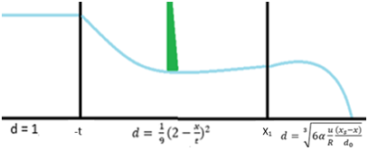
Figure 1 Illustration of the Laminar Flow Regions with their Corresponding Solutions.

During a turbulent dam break event, the ideal fluid flow field yields the following the basic equations. Similar to laminar flow, within its wave tip region the flow velocity does not vary rapidly, hence the influencing concern is not the flow velocity but the wave front celerity, as according to the experimental findings provided from Dressler⁵ and Whitham¹². The wave tip region of the dam break flow under turbulent unsteady conditions for wide channels can be translated to
$f=\frac{1}{d^{\frac{1}{4}}}{\left(3.65x{10}^{-5}{k}_s+\frac{2.5x{10}^{-3}}{R{e}_{d}u}\right)}^{\frac{1}{4}}$                                                                       (13)
The integration of the diffusive equation backward characteristic produces an equation that illustrates the shape of the wave tip region as follows
$d={(\frac{9}{32}{\left(3.65x{10}^{-5}{k}_s+\frac{2.5x{10}^{-3}}{R{e}_{d}u}\right)}^{\frac{1}{4}} u^2\left(x_s-x\right))}^{\frac{4}{9}}$                                                                  (14)
The continuity of the flow properties during the transition between the ideal fluid and wave tip regions is preserved. Hence, the integration of the continuity equation yields the analytical solution below within the context of dimensionless wave front celerity.
$t=\frac{32}{13}\frac{{(1-\frac{u}{2})}^{\frac{7}{2}}}{u^2{\left(3.65x{10}^{-5}{k}_s+\frac{2.5x{10}^{-3}}{R{e}_{d}u}\right)}^{\frac{1}{4}}}$                                                                    (15)
The wave front location is illustrated through equation (16) below, and Figure 2 demonstrates the full flow profile in the presented turbulent model.
$x_s=\left(\frac{3}{2}u-1\right)t+\frac{32}{9}\frac{{(1-\frac{u}{2})}^{\frac{9}{2}}}{u^2{\left(3.65x{10}^{-5}{k}_s+\frac{2.5x{10}^{-3}}{R{e}_{d}u}\right)}^{\frac{1}{4}}}$                                              (16)

Thus, the dimensionless depth satisfies the free surface profiles are
$d=1, at x\le -t$                                                                                                (17)
$d= \frac{1}{9}{(2-\frac{x}{t})}^{2}at -t\le x\le \left(\frac{3}{2}u-1\right)$                                                                          (18)
$d={(\frac{9}{32}{\left(3.65x{10}^{-5}{k}_s+\frac{2.5x{10}^{-3}}{R{e}_{d}u}\right)}^{\frac{1}{4}} u^2\left(x_s-x\right))}^{\frac{4}{9}}at\left(\frac{3}{2}u-1\right)t\le x\le x_s$             (19)
$d=0 at x_s\le x$                                                                                     (20)

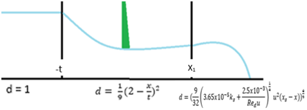
Figure 2 Illustrations of the Turbulent Flow Regions with their Corresponding Solutions.

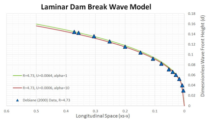
The laminar flow conditions usually used in the published analytical models to reflect flow condition in a large reservoir during the propagation of the dam break wave. To validate the proposed laminar model, this study is concentrated to the in-depth detailed measured data within dam break region to validate its dam break wave computation. In Figure 3 the results of laminar dam break wave model show a positive correlation to the published data. The analytically explicit free-surface profile solutions produces results illustrating accurate the wave front shape as referencing to the measured data provided by Debiane⁴. Also worth noting that different modelling results by various dimensionless velocities are presented in the figure, but make no obvious difference to computed results.

Figure 3 Laminar Dam Break Wave Model versus Debiane⁴ Measured Data.

Debiane⁴ also measured a set of data from their experimental study, which utilized the dimensionless reservoir flow Reynolds Number ‘R’ coefficient as 0.671 and the dimensionless time ‘t’ as 114. In Figure 4 comparison to Debiane4 data, the dimensionless ‘$\frac{x}{t} \text{'}$  is captured within $-7\le \frac{x}{t}\le$ 3.1 due to majority of the wave propagation occurring in this segment during the experiment. The uniform flow velocity recorded by Debiane⁴ was 0.672m/s. Reflected in equations (4),(5) and (11) it can be observed that in order to estimate the wave front analytically a reduction factor $‘\alpha ’$  is required. The reduction factor has proved to be vital in explicitly computing an accurate free surface profile as presenting at Figure 4 and it was observed that adopting $‘\alpha ’$  as 10 increased the model accuracy significantly. In the figure, one can see that by adopting a reduction factor of 1 highly disturbed the accuracy of the model, while utilizing a reduction factor of 100 posed no significant increase in accuracy in comparison to using a reduction factor of 10.

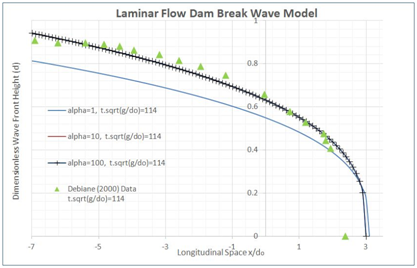
Figure 4Laminar Flow Dam Break Wave Test using Different $\alpha$ Reduction Factor.

The proposed model is also used to produce the turbulent dam break wave results to represent the wave front details reported by experimental data provided by Dressler¹³ and Schoklitsch³. The analytical calculation of the turbulent dam break wave gives efficient solutions with the presences of bed friction as compared to numerical model, i.e. as presented in Pu et al.^6,14. This study also adopts the conceptual model of Whitham¹² in which the ideal fluid flow is used behind the frictionally dominated wave front region. Whitham¹² provided evidence that the analytical dam break wave simulations are unstable at the wave tip, due to the flow singularity with zero water depth hence their study realistically limited to the in-depth detailed data and measurements available on dam break waves in horizontal channels. The published results achieved from the turbulent dam break wave model also indicates that analytical solutions dedicated to dam break waves are suited to flows of high reservoir flow Reynolds Number.²

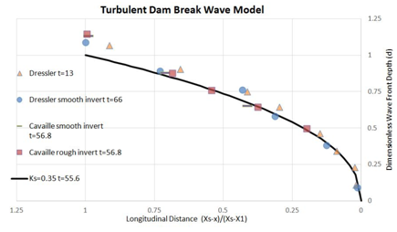
In Figure 5 and Figure 6, the presented model shows a positive correlation with the reported experimental data. The results indicate that the model is dependent on the frictional factor and relative roughness. At the wave tip region located between the wave front start (x₁) and the wave front end (x_s), the inertia acceleration terms are significantly mynute and hence dominated by the flow resistance. Figure 5 illustrates the modelling results computed against the Schoklitsch³ data, which indicated the final wave front location and ideal fluid region is in agreement with published data. It is important to note that the reservoir flow Reynolds Number R was taken as 63000. Dressler⁹ further carried out another experiment, in which the results illustrated the difference between the wave front region of the free surface profile with and without a smooth invert. In order to investigate the measured test case by Dressler⁹, the dimensionless sand roughness height ‘k_s’ has been used in the presented model as 0.35, the dimensionless time ‘t’ was taken as 55.6, and the dimensionless reservoir flow Reynolds Number ‘R’ as 340000 (as the same as conditions in Dressler⁹). The comparison results in Figure 6 shows that the proposed model reproduces the measured turbulent dam break data with good correspondence.

Figure 5 Turbulent Dam Break Wave Model versus Schoklitsch⁴ Measured Data.

Figure 6 Turbulent Dam Break Wave Model versus Dressler¹³ Measured Data.

This study has produced an analytical model to represent the dam break wave by utilizing the explicit modelling suggestions provided by Chanson1,2 for laminar and turbulent flow conditions. In our observation of turbulent modelling, fluids exhibiting low reservoir flow Reynolds Number (Debiane ‘R’=0.671) distorted the results significantly; while fluids exhibiting high reservoir flow Reynolds Number (Dressler ‘R’=340000) provided computation accurately when benchmarked by measurements. It was observed in the laminar dam break wave model that the reduction factor ‘α’ can impact the accuracy of results significantly. The laminar model calculation also indicated that a reduction factor higher than 10 presented no significant increase or decrease in simulation accuracy. It has been noted that the downstream boundary conditions of a dry bed dam break wave decrease to zero at the wave front as the resistance increases to infinity, and this can cause significantly difficult in dam break wave modelling, and approximation used in this studied model has capability to overcome this difficulty and provide precise calculation to the published dam break flow experiments. Generally, all measured data utilized in this study have pointed out that the proposed model is capable to represent different dam break flows under laminar or turbulent flow conditions.¹⁵

None.

Author declares there is no conflict of interest in publishing the article.

1. Chanson H. A Simple Solution of the Laminar Dam Break Wave. Jounral of Applied Fluid Mechanics. 2008;1(1):1−10.
2. Chanson H. A Simple Solution of the Turbulent Dam Break Wave. Journal of Hydraulic Research. 2009;47(1):41−49.
3. Schoklitsch A. Uber Dammbruchwellen. Sitzungsberichte der k. Akademie de Wissenschanfern. 1917;126(IIA):1489−1514.
4. Debiane J. Hydraulique des Ecoulements Laminaires à Surface Libre dans un Canal pour des Milieux Visqueux ou Viscoplastiques: Régimes Uniformes, Graduellement Varié, et Rupture de Barrage. France: Thèse de l’Université Joseph Fourier, Laboratoire de Rhéologie de Grenoble; 2000. 273p.
5. Dressler RF. Comparison of Theories and Experiments for the Hydraulic Dam Break Wave. International Association of Scientific Hydrology Bulletin. 1954;3(38):319–328.
6. Pu JH. Turbulence modelling of shallow water flows using kolmogorov appriach. Computers and Fluids. 2015;115(12):66−74.
7. Zheng XG, Pu JH, Chen R, et al. A Novel Explicit Implicit Coupled Solution Method of SWE for Long-term River Meandering Process Induced by Dambreak. Journal of Applied Fluid Mechanics. 2016;9:2647−2660.
8. Pu JH, Shao S, Huang Y. Numerical and experimental Turbulence Studies on Shallow Open Channel Flows. Journal of Hydro-environment Research. 2014;8(1):9−19.
9. Dressler RF. Hydraulic Resistance Effect Upon the Dam-Break Functions. Journal of Research of the National Bureau of Standards. 1952;49(3):217−225.
10. Deng X, Liu H, Lu S. Analytical Study of Dam-Break Wave Tip Region. Journal of Hydraulic Engineering. 2018;114(5):04018015.
11. Ritter A. Die Fortpflanzung der Wasserwellen. Vereine Deutscher Ingenieure Zeitswchrift. 1892;36(2):947-954.
12. Whitham GB. The Effects of Hydraulic Resistance in The Dam Break Problem. Proceedings of Royal Society, Series A. 1955;227(1170):399–407.
13. Dressler RF, Pohle FV. Resistance Effects on Hydraulic Instability. Communications on Pure and Applied Mathematics. 1953;6:93−96.
14. Pu JH, Lim SY. Efficient numerical computation and experimental study of temporally long equilibrium scour development around abutment. Enviromental Fluid Mechanics. 2014;14(1):69–86.
15. Stoker J. Water Waves: The Mathematical Theory with Applications. New York: Interscience Publishers; 1957. 609p.