Submit manuscript...
eISSN: 2641-936X

Electrical & Electronic Technology Open Access Journal

Mini Review Volume 2 Issue 5

Molecular communication noise effect analysis of diffusion based channel for considering msk and mosk modulations

A Azari, SK Seyyedi S

Department of Electrical Engineering, Islamic Azad University, Iran

Correspondence: A Azari, Department of Electrical Engineering, Islamic Azad University, Iran,

Received: August 18, 2017 | Published: November 28, 2018

Citation: Azari A, Seyyedi SKS. Molecular communication noise effect analysis of diffusion based channel for considering msk and mosk modulations. Electric Electron Tech Open Acc J. 2018;2(5):317-320. DOI: 10.15406/eetoaj.2018.02.00035

Download PDF

Abstract

One of the unaddressed and open challenges in the nano-networking is the characterstics of noise. The previous analysis, however, have concentrated on end-to-end communication model with no separate modelings for propagation channel and noise. By considering a separate signal propagation and noise model, the design and implementation of an optimum receiver will be much easier. In this paper we justify consideration of a separate additive Gaussian noise model of a nano-communication system based on the molecular communication channel for which are applicable for Msk and Mosk modulation schemes. The presented noise analysis is based on the Brownian motion process and advection molecular statistics, where the received random signal has a probability density function whose mean is equal to the mean number of the received molecules. Finally, the justification of received signal magnitude being uncorrelated with additive non-stationary white noise, is provided.

Keywords: molecular, noise, diffusion, channel, frequency shift keying

Introduction

Any molecular communication model similar to conventional digital communication system consist of three main components, they are the transmitter, receiver, and the channel. Figure 1 illustrates a schematic of a molecular communication model. In comparison with the digital communication system model, molecular communication system can also be implemented using different types of modulation schemes. The modulation techniques mainly used in digital communications.1 Pulse Amplitude Modulation (PAM), Phase Shift Keying (PSK), and Frequency Shift Keying (FSK). In PAM, different amplitudes are used for message modulation. In PSK, to modulate different messages finite number of phases are used, and in FSK, finite number of frequencies are used for modulating the messages.
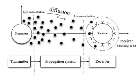
Figure 1 A schematic of a molecular communication system.

Considering nano-communication transmission and reception environment as shown in Figure 2 in general, transmitters can employ three modulation techniques:

Concentration Shift Keying (CSK), which is similar to PAM. In this type of modulation, only one type of molecule is used and messages are encoded by different amounts of released molecules.2–5

Pulse Position Modulation (PPM), where only on type of molecule is used and messages are encoded by transmitting single pulse in different time shifts.6,7

Molecular Shift Keying (MOSK), in which messages are encoded by using different type of molecules.8,9 To avoid interference the signal space will be chosen to be orthogonal. In10 it is shown that this type of modulation in comparison to CSK is more robust against noise.

Figure 2 Block diagram of a molecular communication system.

The modeling and characterization of noise in a conventional communication is well defined and very broadly analyzed. But in contrast to this, in the molecular communications characterization of noise still one of the open challenges for researchers. Even though, noise sources of molecular communications are analyzed in terms of stochastic process, but most of the works have concentrated on a general end-to-end communication model with considering no separate model for the propagation channel and noise. It is then believed that, by having a separate signal propagation and noise model, if one wants to follow, the design of an optimum receiver will be much easier task.

Noise modeling in diffusion-based molecular communication

Consider the diffusion –based noisy channel of Figure 3; where at time zero ,Q number of messenger molecules are propagated through the diffusion channel of impulse response h(t). Let n(t) be the sample function of a noise random process N(t) , then due to the nature of the channel ,that is the diffusion channel ,it is not hard to see that we may be able to consider two different types of noises .That is nb(t) and nr(t) are being the Brownian and Residual noises respectively (Figure 4).
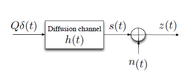
Figure 3 Diffusion-based molecular channel model.
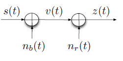
Figure 4 Model of the two separate noise components.

It is worth to know that, nb(t) ,the Brownian noise is associated with the random thermal motion of the messenger molecules and nr(t), the residual noise ,is as a result of the interference due to the messenger molecules. We also should remind that nr(t) is analogous to the inter–symbol interferences in the conventional communications. Now, considering z(t) being the input to the receiver or the output of the channel, we might be able to write

Z(t)= s(t)+ nb(t)+ nr(t)                           (1)

Where s(t) is the mean number of the received messenger molecules.

Brownian noise in diffusion-based molecular channel

Since Brownian noise is produced by the random thermal motion of the transmitted messenger molecules, then the number of counted molecules at the receiver are random. Let X(t) = (x(t),y(t),z(t)) be a three dimensional position of a messenger molecule at time, t, since the Brownian motion is modeled by the Wiener process, for a two dimensional reception surface, we may write,

x(t)= x + 2Dt u(t) y(t)= y + 2Dt u(t) MathType@MTEF@5@5@+= feaagKart1ev2aaatCvAUfeBSjuyZL2yd9gzLbvyNv2CaerbuLwBLn hiov2DGi1BTfMBaeXatLxBI9gBaerbd9wDYLwzYbItLDharqqtubsr 4rNCHbGeaGqiVu0Je9sqqrpepC0xbbL8F4rqqrFfpeea0xe9Lq=Jc9 vqaqpepm0xbba9pwe9Q8fs0=yqaqpepae9pg0FirpepeKkFr0xfr=x fr=xb9adbaqaaeGaciGaaiaabeqaamaabaabaaGceaqabeaajugibi aadIhacaGGOaGaamiDaiaacMcacqGH9aqpcaaMc8Ecfa4aaCbiaOqa aKqzGeGaamiEaaWcbeqaaKqzGeGaey4jIKnaaiabgUcaRKqbaoaaka aakeaajugibiaaikdacaWGebGaamiDaaWcbeaajugibiaaykW7caWG 1bGaaiikaiaadshacaGGPaGaaGPaVdGcbaqcLbsacaWG5bGaaiikai aadshacaGGPaGaeyypa0JaaGPaVNqbaoaaxacakeaajugibiaadMha aSqabeaajugibiabgEIizdaacqGHRaWkjuaGdaGcaaGcbaqcLbsaca aIYaGaamiraiaadshaaSqabaqcLbsacaaMc8UaamyDaiaacIcacaWG 0bGaaiykaiaaykW7aaaa@6361@                               (2)

where (x,y) being the original position of the transmitted messenger molecular with u(t) having a standarized normal distribution, u(t) ~ N(0,1). Therefore, for, any fixed t=t0, the mean or expected values of x(t0) and y(t0 ) are given respectively by ;

E(x( t 0 ))= x + 2D t 0 E(U( t 0 ))= x E(y( t 0 ))= y + 2D t 0 E(U( t 0 ))= y MathType@MTEF@5@5@+= feaagKart1ev2aaatCvAUfeBSjuyZL2yd9gzLbvyNv2CaerbuLwBLn hiov2DGi1BTfMBaeXatLxBI9gBaerbd9wDYLwzYbItLDharqqtubsr 4rNCHbGeaGqiVu0Je9sqqrpepC0xbbL8F4rqqrFfpeea0xe9Lq=Jc9 vqaqpepm0xbba9pwe9Q8fs0=yqaqpepae9pg0FirpepeKkFr0xfr=x fr=xb9adbaqaaeGaciGaaiaabeqaamaabaabaaGceaqabeaajugibi aadweacaGGOaGaamiEaiaacIcacaWG0bWcdaWgaaqaaKqzadGaaGim aaWcbeaajugibiaacMcacaGGPaGaeyypa0JaaGPaVVWaaCbiaOqaaK qzadGaamiEaaWcbeqaaKqzadGaey4jIKnaaKqzGeGaey4kaSscfa4a aOaaaOqaaKqzGeGaaGOmaiaadseacaWG0bWcdaWgaaqaaKqzadGaaG imaaWcbeaaaeqaaKqzGeGaaGPaVlaadweacaGGOaGaamyvaiaacIca caWG0bWcdaWgaaqaaKqzadGaaGimaaWcbeaajugibiaacMcacaGGPa GaaGPaVlabg2da9iaaykW7juaGdaWfGaGcbaqcLbsacaWG4baaleqa baqcLbmacqGHNis2aaaakeaajugibiaadweacaGGOaGaamyEaiaacI cacaWG0bWcdaWgaaqaaKqzadGaaGimaaWcbeaajugibiaacMcacaGG PaGaeyypa0tcfa4aaCbiaOqaaKqzGeGaamyEaaWcbeqaaKqzadGaey 4jIKnaaKqzGeGaaGPaVlabgUcaRKqbaoaakaaakeaajugibiaaikda caWGebGaamiDaKqbaoaaBaaaleaajugWaiaaicdaaSqabaaabeaaju gibiaaykW7caWGfbGaaiikaiaadwfacaGGOaGaamiDaSWaaSbaaeaa jugWaiaaicdaaSqabaqcLbsacaGGPaGaaiykaiaaykW7cqGH9aqpca aMc8Ecfa4aaCbiaOqaaKqzGeGaamyEaaWcbeqaaKqzadGaey4jIKna aaaaaa@8D48@                                                                       (3)

and as a result, for each emitted molecule ,the joint probability density function of being at point (x(t),y(t)), Pxy (x(t),y(t)) is a two dimensional Guassian distribution function , where

P xy (x(t),y(t))= P x (x(t)) P y (y(t))= 1 4πDt exp( (x(t) x ) 2 + (y(t) y ) 2 4Dt ) MathType@MTEF@5@5@+= feaagKart1ev2aaatCvAUfeBSjuyZL2yd9gzLbvyNv2CaerbuLwBLn hiov2DGi1BTfMBaeXatLxBI9gBaerbd9wDYLwzYbItLDharqqtubsr 4rNCHbGeaGqiVu0Je9sqqrpepC0xbbL8F4rqqrFfpeea0xe9Lq=Jc9 vqaqpepm0xbba9pwe9Q8fs0=yqaqpepae9pg0FirpepeKkFr0xfr=x fr=xb9adbaqaaeGaciGaaiaabeqaamaabaabaaGcbaqcLbsacaWGqb qcfa4aaSbaaSqaaKqzadGaamiEaiaadMhaaSqabaqcLbsacaGGOaGa amiEaiaacIcacaWG0bGaaiykaiaacYcacaWG5bGaaiikaiaadshaca GGPaGaaiykaiaaykW7cqGH9aqpcaaMc8UaamiuaKqbaoaaBaaaleaa jugWaiaadIhaaSqabaqcLbsacaGGOaGaamiEaiaacIcacaWG0bGaai ykaiaacMcacaWGqbqcfa4aaSbaaSqaaKqzadGaamyEaaWcbeaajugi biaacIcacaWG5bGaaiikaiaadshacaGGPaGaaiykaiaaykW7cqGH9a qpcaaMc8Ecfa4aaSaaaOqaaKqzGeGaaGymaaGcbaqcLbsacaaI0aGa eqiWdaNaamiraiaadshaaaGaciyzaiaacIhacaGGWbGaaiikaiabgk HiTKqbaoaalaaakeaajugibiaacIcacaWG4bGaaiikaiaadshacaGG PaGaeyOeI0scfa4aaCbiaOqaaKqzGeGaamiEaaWcbeqaaKqzadGaey 4jIKnaaKqzGeGaaiykaKqbaoaaCaaaleqabaqcLbmacaaIYaaaaKqz GeGaaGPaVlabgUcaRiaacIcacaWG5bGaaiikaiaadshacaGGPaGaaG PaVlabgkHiTiaaykW7juaGdaWfGaGcbaqcLbsacaWG5baaleqabaqc LbmacqGHNis2aaqcLbsacaGGPaWcdaahaaqabeaajugWaiaaikdaaa aakeaajugibiaaisdacaWGebGaamiDaaaacaGGPaaaaa@9094@                  (4)

with mean ( x^(t),y^(t) ) and variance 2Dt, with D being the diffusion coefficient. Hence the probability of having a messenger molecule in the sensing surface area of Ar is given by:

P= A r P xy (x(t),y(t))dxdy = A r 1 4πDt exp( (x(t) x ) 2 + (y(t) y ) 2 4Dt )dxdy MathType@MTEF@5@5@+= feaagKart1ev2aaatCvAUfeBSjuyZL2yd9gzLbvyNv2CaerbuLwBLn hiov2DGi1BTfMBaeXatLxBI9gBaerbd9wDYLwzYbItLDharqqtubsr 4rNCHbGeaGqiVu0Je9sqqrpepC0xbbL8F4rqqrFfpeea0xe9Lq=Jc9 vqaqpepm0xbba9pwe9Q8fs0=yqaqpepae9pg0FirpepeKkFr0xfr=x fr=xb9adbaqaaeGaciGaaiaabeqaamaabaabaaGcbaqcLbsacaWGqb Gaeyypa0tcfa4aa8GuaOqaaKqzGeGaamiuaSWaaSbaaeaajugWaiaa dIhacaWG5baaleqaaKqzGeGaaiikaiaadIhacaGGOaGaamiDaiaacM cacaGGSaGaamyEaiaacIcacaWG0bGaaiykaiaacMcacaWGKbGaamiE aiaadsgacaWG5baaleaajugibiaadgeajuaGdaWgaaadbaqcLbsaca WGYbaameqaaaWcbeqcLbsacqGHRiI8cqGHRiI8aiaaykW7cqGH9aqp juaGdaWdsbGcbaqcfa4aaSaaaOqaaKqzGeGaaGymaaGcbaqcLbsaca aI0aGaeqiWdaNaamiraiaadshaaaaaleaajugibiaadgeajuaGdaWg aaadbaqcLbmacaWGYbaameqaaaWcbeqcLbsacqGHRiI8cqGHRiI8ai GacwgacaGG4bGaaiiCaiaacIcacqGHsisljuaGdaWcaaGcbaqcLbsa caGGOaGaamiEaiaacIcacaWG0bGaaiykaiabgkHiTKqbaoaaxacake aajugibiaadIhaaSqabeaajugWaiabgEIizdaajugibiaacMcajuaG daahaaWcbeqaaKqzadGaaGOmaaaajugibiaaykW7cqGHRaWkcaGGOa GaamyEaiaacIcacaWG0bGaaiykaiaaykW7cqGHsislcaaMc8Ecfa4a aCbiaOqaaKqzGeGaamyEaaWcbeqaaKqzadGaey4jIKnaaKqzGeGaai ykaSWaaWbaaeqabaqcLbmacaaIYaaaaaGcbaqcLbsacaaI0aGaamir aiaadshaaaGaaiykaiaadsgacaWG4bGaamizaiaadMhaaaa@94C2@                  (5)

Let us now, assume that Q messenger molecules are emitted by the transmitter of the nano-system , then the reception of K messenger molecules in the sensing area of the receiver has Binomial distribution with probability mass function given by:

P(k)=( Q k )( k P ) (1P) Qk MathType@MTEF@5@5@+= feaagKart1ev2aaatCvAUfeBSjuyZL2yd9gzLbvyNv2CaerbuLwBLn hiov2DGi1BTfMBaeXatLxBI9gBaerbd9wDYLwzYbItLDharqqtubsr 4rNCHbGeaGqiVu0Je9sqqrpepC0xbbL8F4rqqrFfpeea0xe9Lq=Jc9 vqaqpepm0xbba9pwe9Q8fs0=yqaqpepae9pg0FirpepeKkFr0xfr=x fr=xb9adbaqaaeGaciGaaiaabeqaamaabaabaaGcbaqcLbsacaWGqb GaaiikaiaadUgacaGGPaGaeyypa0tcfa4aaeWaaKqzGeabaeqakeaa jugibiaadgfaaOqaaKqzGeGaam4AaaaakiaawIcacaGLPaaajuaGda qadaqcLbsaeaqabOqaaKqzGeGaam4AaaGcbaqcLbsacaWGqbaaaOGa ayjkaiaawMcaaKqzGeGaaiikaiaaigdacqGHsislcaWGqbGaaiykaS WaaWbaaeqabaqcLbmacaWGrbGaeyOeI0Iaam4Aaaaaaaa@4E79@                                                          (6)

As we know, if we choose Q large and p small enough ,then the Eq.(6),can be approximated by a Gaussian distribution N(μ, σ 2 ) MathType@MTEF@5@5@+= feaagKart1ev2aaatCvAUfeBSjuyZL2yd9gzLbvyNv2CaerbuLwBLn hiov2DGi1BTfMBaeXatLxBI9gBaerbd9wDYLwzYbItLDharqqtubsr 4rNCHbGeaGqiVu0Je9sqqrpepC0xbbL8F4rqqrFfpeea0xe9Lq=Jc9 vqaqpepm0xbba9pwe9Q8fs0=yqaqpepae9pg0FirpepeKkFr0xfr=x fr=xb9adbaqaaeGaciGaaiaabeqaamaabaabaaGcbaqcLbsacaWGob GaaiikaiabeY7aTjaacYcacqaHdpWCjuaGdaahaaWcbeqaaKqzadGa aGOmaaaajugibiaacMcaaaa@400E@  where μ=QP MathType@MTEF@5@5@+= feaagKart1ev2aaatCvAUfeBSjuyZL2yd9gzLbvyNv2CaerbuLwBLn hiov2DGi1BTfMBaeXatLxBI9gBaerbd9wDYLwzYbItLDharqqtubsr 4rNCHbGeaGqiVu0Je9sqqrpepC0xbbL8F4rqqrFfpeea0xe9Lq=Jc9 vqaqpepm0xbba9pwe9Q8fs0=yqaqpepae9pg0FirpepeKkFr0xfr=x fr=xb9adbaqaaeGaciGaaiaabeqaamaabaabaaGcbaqcLbsacqaH8o qBcqGH9aqpcaWGrbGaamiuaaaa@3AEC@  and σ 2 =QP(1P) MathType@MTEF@5@5@+= feaagKart1ev2aaatCvAUfeBSjuyZL2yd9gzLbvyNv2CaerbuLwBLn hiov2DGi1BTfMBaeXatLxBI9gBaerbd9wDYLwzYbItLDharqqtubsr 4rNCHbGeaGqiVu0Je9sqqrpepC0xbbL8F4rqqrFfpeea0xe9Lq=Jc9 vqaqpepm0xbba9pwe9Q8fs0=yqaqpepae9pg0FirpepeKkFr0xfr=x fr=xb9adbaqaaeGaciGaaiaabeqaamaabaabaaGcbaqcLbsacqaHdp WClmaaCaaabeqaaKqzadGaaGOmaaaajugibiabg2da9iaadgfacaWG qbGaaiikaiaaigdacqGHsislcaWGqbGaaiykaaaa@4175@ . By combining of the Eqs.(5 ,6 ) , we get the result

μ=QP=Q A r 1 4πDt exp( (x(t) x ) 2 + (y(t) y ) 2 4Dt )dxdy MathType@MTEF@5@5@+= feaagKart1ev2aaatCvAUfeBSjuyZL2yd9gzLbvyNv2CaerbuLwBLn hiov2DGi1BTfMBaeXatLxBI9gBaerbd9wDYLwzYbItLDharqqtubsr 4rNCHbGeaGqiVu0Je9sqqrpepC0xbbL8F4rqqrFfpeea0xe9Lq=Jc9 vqaqpepm0xbba9pwe9Q8fs0=yqaqpepae9pg0FirpepeKkFr0xfr=x fr=xb9adbaqaaeGaciGaaiaabeqaamaabaabaaGcbaqcLbsacqaH8o qBcqGH9aqpcaWGrbGaamiuaiabg2da9iaadgfajuaGdaWdsbGcbaqc fa4aaSaaaOqaaKqzGeGaaGymaaGcbaqcLbsacaaI0aGaeqiWdaNaam iraiaadshaaaaaleaajugibiaadgealmaaBaaameaajugWaiaadkha aWqabaaaleqajugibiabgUIiYlabgUIiYdGaciyzaiaacIhacaGGWb GaaiikaiabgkHiTKqbaoaalaaakeaajugibiaacIcacaWG4bGaaiik aiaadshacaGGPaGaeyOeI0scfa4aaCbiaOqaaKqzGeGaamiEaaWcbe qaaKqzadGaey4jIKnaaKqzGeGaaiykaSWaaWbaaeqabaqcLbmacaaI YaaaaKqzGeGaaGPaVlabgUcaRiaacIcacaWG5bGaaiikaiaadshaca GGPaGaaGPaVlabgkHiTiaaykW7juaGdaWfGaGcbaqcLbsacaWG5baa leqabaqcLbmacqGHNis2aaqcLbsacaGGPaWcdaahaaqabeaajugWai aaikdaaaaakeaajugibiaaisdacaWGebGaamiDaaaacaGGPaGaamiz aiaadIhacaWGKbGaamyEaaaa@7AE3@                 (7)

Comparing the mean value u in the Eq.(7) with the Eq.(5) ,it is not hard to see that these two quantities are the same ,that is u is the same as the mean number of received messenger molecules . This implies that the received random signal has a probability density function whose mean is the deterministic signal of the Eq.(5).Thus this equality justifies the facts that first, Brownian noise is additive, second signal in Eq.(5) is the response of the molecular channel. Let v(t) be the number of the messenger molecules corrupted by Brownian noise , as shown in Figure 5, to be defined as follows;

v(t)=s(t)+ n b (t) MathType@MTEF@5@5@+= feaagKart1ev2aaatCvAUfeBSjuyZL2yd9gzLbvyNv2CaerbuLwBLn hiov2DGi1BTfMBaeXatLxBI9gBaerbd9wDYLwzYbItLDharqqtubsr 4rNCHbGeaGqiVu0Je9sqqrpepC0xbbL8F4rqqrFfpeea0xe9Lq=Jc9 vqaqpepm0xbba9pwe9Q8fs0=yqaqpepae9pg0FirpepeKkFr0xfr=x fr=xb9adbaqaaeGaciGaaiaabeqaamaabaabaaGcbaqcLbsacaWG2b GaaiikaiaadshacaGGPaGaeyypa0Jaam4CaiaacIcacaWG0bGaaiyk aiaaykW7cqGHRaWkcaWGUbWcdaWgaaqaaKqzadGaamOyaaWcbeaaju gibiaacIcacaWG0bGaaiykaaaa@46AF@                                                                   (8)

then, v(t) has Gaussian distribution of mean s(t) and variance QP(1-P), that is N(s(t),QP(1-P)). So, v(t)-s(t)=nb( (t) has distribution of N(0,p(1-p)). Now if we assume p<<1, then we can say that  1-p~1 and only then the var( n b )= σ 2 nb QP MathType@MTEF@5@5@+= feaagKart1ev2aaatCvAUfeBSjuyZL2yd9gzLbvyNv2CaerbuLwBLn hiov2DGi1BTfMBaeXatLxBI9gBaerbd9wDYLwzYbItLDharqqtubsr 4rNCHbGeaGqiVu0Je9sqqrpepC0xbbL8F4rqqrFfpeea0xe9Lq=Jc9 vqaqpepm0xbba9pwe9Q8fs0=yqaqpepae9pg0FirpepeKkFr0xfr=x fr=xb9adbaqaaeGaciGaaiaabeqaamaabaabaaGcbaqcLbsaciGG2b GaaiyyaiaackhacaGGOaGaamOBaSWaaSbaaeaajugWaiaadkgaaSqa baqcLbsacaGGPaGaeyypa0Jaeq4Wdm3cdaahaaqabeaajugWaiaaik daaaqcfa4aaSbaaSqaaKqzadGaamOBaiaadkgaaSqabaqcLbsacqGH ijYUcaWGrbGaamiuaaaa@4B1B@ . We also Know that QP=E(S(t)) and thus n b (t)=( s(t) )N(0,1) MathType@MTEF@5@5@+= feaagKart1ev2aaatCvAUfeBSjuyZL2yd9gzLbvyNv2CaerbuLwBLn hiov2DGi1BTfMBaeXatLxBI9gBaerbd9wDYLwzYbItLDharqqtubsr 4rNCHbGeaGqiVu0Je9sqqrpepC0xbbL8F4rqqrFfpeea0xe9Lq=Jc9 vqaqpepm0xbba9pwe9Q8fs0=yqaqpepae9pg0FirpepeKkFr0xfr=x fr=xb9adbaqaaeGaciGaaiaabeqaamaabaabaaGcbaqcLbsacaWGUb qcfa4aaSbaaSqaaKqzadGaamOyaaWcbeaajugibiaacIcacaWG0bGa aiykaiabg2da9iaacIcajuaGdaGcaaGcbaqcLbsacaWGZbGaaiikai aadshacaGGPaaaleqaaKqzGeGaaiykaiaad6eacaGGOaGaaGimaiaa cYcacaaIXaGaaiykaaaa@48FE@ , which implies that Brownian noise follows a zero mean Gaussian process with variance equal to the mean number of received molecules in the sensing area. To investigate the statistical properties of the Brownian noise we want to compute the autocorrelation function of the Brownian noise, that is Rnb (t1 ,t2 ). Since the probability density function of the Brownian noise is derived through the probability density function of v(t), lets compute the second order density function of v(t). Using the chain rule of probability,

P V ( v 1 , v 2 )=P( v 2 | v 1 )P( v 1 )=P( v 1 | v 2 )P( v 2 ) MathType@MTEF@5@5@+= feaagKart1ev2aaatCvAUfeBSjuyZL2yd9gzLbvyNv2CaerbuLwBLn hiov2DGi1BTfMBaeXatLxBI9gBaerbd9wDYLwzYbItLDharqqtubsr 4rNCHbGeaGqiVu0Je9sqqrpepC0xbbL8F4rqqrFfpeea0xe9Lq=Jc9 vqaqpepm0xbba9pwe9Q8fs0=yqaqpepae9pg0FirpepeKkFr0xfr=x fr=xb9adbaqaaeGaciGaaiaabeqaamaabaabaaGcbaqcLbsacaWGqb WcdaWgaaqaaKqzadGaamOvaaWcbeaajugibiaacIcacaWG2bWcdaWg aaqaaKqzadGaaGymaaWcbeaajugibiaacYcacaWG2bWcdaWgaaqaaK qzadGaaGOmaaWcbeaajugibiaacMcacqGH9aqpcaWGqbGaaiikaiaa dAhajuaGdaWgaaWcbaqcLbmacaaIYaaaleqaaKqbaoaaeeaakeaaju gibiaadAhalmaaBaaabaqcLbmacaaIXaaaleqaaaGccaGLhWoajugi biaacMcacaWGqbGaaiikaiaadAhalmaaBaaabaqcLbmacaaIXaaale qaaKqzGeGaaiykaiabg2da9iaadcfacaGGOaGaamODaSWaaSbaaeaa jugWaiaaigdaaSqabaqcfa4aaqqaaOqaaKqzGeGaamODaKqbaoaaBa aaleaajugWaiaaikdaaSqabaaakiaawEa7aKqzGeGaaiykaiaadcfa caGGOaGaamODaSWaaSbaaeaajugWaiaaikdaaSqabaqcLbsacaGGPa aaaa@69D2@                       (9)

with vi =v(ti ) for i=1,2. According to Eq.(6) vi is a binomial random variable with parameters Q,P, B(Q,P) , with p1 being the probability of Q messenger molecules at the receiving area at time t1. The same argument is true for the v(t2)=v2. But p(V2/V1) ,the probability of having v2 molecules at the receiving area at time t2 given that v1 molecules have been transmitted at time t1 where t1<t2, we then can write.

P V ( v 2 | v 1 )= i=0 v 1 (inumberof v 1 moleculesarestayinginthesenseingarea)P( v 2 inewmoleculesarecoming) = i=0 v 1 P st (i) P na (i) MathType@MTEF@5@5@+= feaagKart1ev2aaatCvAUfeBSjuyZL2yd9gzLbvyNv2CaerbuLwBLn hiov2DGi1BTfMBaeXatLxBI9gBaerbd9wDYLwzYbItLDharqqtubsr 4rNCHbGeaGqiVu0Je9sqqrpepC0xbbL8F4rqqrFfpeea0xe9Lq=Jc9 vqaqpepm0xbba9pwe9Q8fs0=yqaqpepae9pg0FirpepeKkFr0xfr=x fr=xb9adbaqaaeGaciGaaiaabeqaamaabaabaaGceaqabeaajugibi aadcfalmaaBaaabaqcLbmacaWGwbaaleqaaKqzGeGaaiikaiaadAha lmaaBaaabaqcLbmacaaIYaaaleqaaKqbaoaaeeaakeaajugibiaadA halmaaBaaabaqcLbmacaaIXaaaleqaaKqzGeGaaiykaiaaykW7aOGa ay5bSdqcLbsacqGH9aqpjuaGdaaeWbGcbaqcLbsacaGGOaGaamyAai aaykW7caWGUbGaamyDaiaad2gacaWGIbGaamyzaiaadkhacaaMc8Ua am4BaiaadAgacaaMc8UaamODaSWaaSbaaeaajugWaiaaigdaaSqaba qcLbsacaaMc8UaamyBaiaad+gacaWGSbGaamyzaiaadogacaWG1bGa amiBaiaadwgacaWGZbGaaGPaVlaadggacaWGYbGaamyzaiaaykW7ca WGZbGaamiDaiaadggacaWG5bGaamyAaiaad6gacaWGNbGaaGPaVlaa dMgacaWGUbGaaGPaVlaadshacaWGObGaamyzaiaaykW7caWGZbGaam yzaiaad6gacaWGZbGaamyzaiaadMgacaWGUbGaam4zaiaaykW7caWG HbGaamOCaiaadwgacaWGHbGaaiykaiaadcfacaGGOaGaamODaSWaaS baaeaajugWaiaaikdaaSqabaqcLbsacqGHsislcaWGPbGaaGPaVlaa d6gacaWGLbGaam4DaiaaykW7caWGTbGaam4BaiaadYgacaWGLbGaam 4yaiaadwhacaWGSbGaamyzaiaadohacaaMc8UaamyyaiaadkhacaWG LbGaaGPaVlaadogacaWGVbGaciyBaiaacMgacaGGUbGaam4zaiaacM caaSqaaKqzadGaamyAaiabg2da9iaaicdaaSqaaKqzadGaamODaSWa aSbaaWqaaKqzadGaaGymaaadbeaaaKqzGeGaeyyeIuoaaOqaaKqzGe GaaGPaVlaaykW7caaMc8UaaGPaVlaaykW7caaMc8UaaGPaVlaaykW7 caaMc8UaaGPaVlaaykW7caaMc8UaaGPaVlaaykW7caaMc8UaaGPaVl aaykW7caaMc8UaaGPaVlaaykW7caaMc8Uaeyypa0JaaGPaVNqbaoaa qahakeaajugibiaadcfalmaaBaaabaqcLbmacaWGZbGaamiDaaWcbe aajugibiaacIcacaWGPbGaaiykaiaadcfajuaGdaWgaaWcbaqcLbma caWGUbGaamyyaaWcbeaajugibiaacIcacaWGPbGaaiykaaWcbaqcLb macaWGPbGaeyypa0JaaGimaaWcbaqcLbmacaWG2bWcdaWgaaadbaqc LbmacaaIXaaameqaaaqcLbsacqGHris5aaaaaa@F2C3@  (10)

where pst(i) =p( i number of v1 molecules staying in the sensing area) and is given by

P st (i)=( v 1 i )( i p 2 ) ( 1 p 2 ) v 1 i MathType@MTEF@5@5@+= feaagKart1ev2aaatCvAUfeBSjuyZL2yd9gzLbvyNv2CaerbuLwBLn hiov2DGi1BTfMBaeXatLxBI9gBaerbd9wDYLwzYbItLDharqqtubsr 4rNCHbGeaGqiVu0Je9sqqrpepC0xbbL8F4rqqrFfpeea0xe9Lq=Jc9 vqaqpepm0xbba9pwe9Q8fs0=yqaqpepae9pg0FirpepeKkFr0xfr=x fr=xb9adbaqaaeGaciGaaiaabeqaamaabaabaaGcbaqcLbsacaWGqb qcfa4aaSbaaSqaaKqzadGaam4CaiaadshaaSqabaqcLbsacaGGOaGa amyAaiaacMcacaaMc8Uaeyypa0JaaGPaVNqbaoaabmaajugibqaabe GcbaqcLbsacaWG2bWcdaWgaaqaaKqzadGaaGymaaWcbeaaaOqaaKqz GeGaamyAaaaakiaawIcacaGLPaaajuaGdaqadaqcLbsaeaqabOqaaK qzGeGaamyAaaGcbaqcLbsacaWGWbWcdaWgaaqaaKqzadGaaGOmaaWc beaaaaGccaGLOaGaayzkaaqcfa4aaeWaaOqaaKqzGeGaaGymaiabgk HiTiaadchajuaGdaWgaaWcbaqcLbmacaaIYaaaleqaaaGccaGLOaGa ayzkaaqcfa4aaWbaaSqabeaajugibiaadAhalmaaBaaameaajugWai aaigdaaWqabaqcLbsacqGHsislcaWGPbaaaaaa@60F1@                              (11)

where p2, being the probability of an event a messenger molecule staying in the receiving area after t2 –t1 seconds passed. Also, if we let p(v2 –i new molecules are arriving ) =pna(t), then

P na (i)=( Q v 1 v 2 i )( v 2 i p 3 ) ( 1 p 3 ) (Q v 1 )( v 2 i) MathType@MTEF@5@5@+= feaagKart1ev2aaatCvAUfeBSjuyZL2yd9gzLbvyNv2CaerbuLwBLn hiov2DGi1BTfMBaeXatLxBI9gBaerbd9wDYLwzYbItLDharqqtubsr 4rNCHbGeaGqiVu0Je9sqqrpepC0xbbL8F4rqqrFfpeea0xe9Lq=Jc9 vqaqpepm0xbba9pwe9Q8fs0=yqaqpepae9pg0FirpepeKkFr0xfr=x fr=xb9adbaqaaeGaciGaaiaabeqaamaabaabaaGcbaqcLbsacaWGqb WcdaWgaaqaaKqzadGaamOBaiaadggaaSqabaqcLbsacaGGOaGaamyA aiaacMcacaaMc8Uaeyypa0JaaGPaVNqbaoaabmaajugibqaabeGcba qcLbsacaWGrbGaeyOeI0IaamODaSWaaSbaaeaajugWaiaaigdaaSqa baaakeaajugibiaadAhalmaaBaaabaqcLbmacaaIYaaaleqaaKqzGe GaeyOeI0IaamyAaaaakiaawIcacaGLPaaajuaGdaqadaqcLbsaeaqa bOqaaKqzGeGaamODaKqbaoaaBaaaleaajugibiaaikdaaSqabaqcLb sacqGHsislcaWGPbaakeaajugibiaadchalmaaBaaabaqcLbmacaaI ZaaaleqaaaaakiaawIcacaGLPaaajuaGdaqadaGcbaqcLbsacaaIXa GaeyOeI0IaamiCaKqbaoaaBaaaleaajugWaiaaiodaaSqabaaakiaa wIcacaGLPaaajuaGdaahaaWcbeqaaKqzGeGaaiikaiaadgfacqGHsi slcaWG2bWcdaWgaaadbaqcLbmacaaIXaaameqaaKqzGeGaaiykaiab gkHiTiaacIcacaWG2bqcfa4aaSbaaWqaaKqzadGaaGOmaaadbeaaju gibiabgkHiTiaadMgacaGGPaaaaaaa@74CC@ (12)

which is a binomial probability function , with p3 being the probability of having a messenger molecule at the sensing area at time t2. Now by considering the fact that for Q>>v1 , then Q-V1 ~ Q, we can write.

P na (i)=( Q v 2 i )( v 2 i p 3 ) ( 1 p 3 ) Q( v 2 i) MathType@MTEF@5@5@+= feaagKart1ev2aaatCvAUfeBSjuyZL2yd9gzLbvyNv2CaerbuLwBLn hiov2DGi1BTfMBaeXatLxBI9gBaerbd9wDYLwzYbItLDharqqtubsr 4rNCHbGeaGqiVu0Je9sqqrpepC0xbbL8F4rqqrFfpeea0xe9Lq=Jc9 vqaqpepm0xbba9pwe9Q8fs0=yqaqpepae9pg0FirpepeKkFr0xfr=x fr=xb9adbaqaaeGaciGaaiaabeqaamaabaabaaGcbaqcLbsacaWGqb WcdaWgaaqaaKqzadGaamOBaiaadggaaSqabaqcLbsacaGGOaGaamyA aiaacMcacaaMc8Uaeyypa0JaaGPaVNqbaoaabmaajugibqaabeGcba qcLbsacaWGrbaakeaajugibiaadAhalmaaBaaabaqcLbmacaaIYaaa leqaaKqzGeGaeyOeI0IaamyAaaaakiaawIcacaGLPaaajuaGdaqada qcLbsaeaqabOqaaKqzGeGaamODaSWaaSbaaeaajugWaiaaikdaaSqa baqcLbsacqGHsislcaWGPbaakeaajugibiaadchalmaaBaaabaqcLb macaaIZaaaleqaaaaakiaawIcacaGLPaaajuaGdaqadaGcbaqcLbsa caaIXaGaeyOeI0IaamiCaKqbaoaaBaaaleaajugWaiaaiodaaSqaba aakiaawIcacaGLPaaajuaGdaahaaWcbeqaaKqzGeGaamyuaiabgkHi TiaacIcacaWG2bWcdaWgaaadbaqcLbmacaaIYaaameqaaKqzGeGaey OeI0IaamyAaiaacMcaaaaaaa@6A55@         (13)

By assuming the remaining i molecules in the sensing area is negligible, that is i=0 , the Eq.(7) will become

P( v 2 | v 1 ) P na (i=0)=( Q v 2 )( v 2 p 3 ) ( 1 p 3 ) Q v 2 =Pv( v 2 ) MathType@MTEF@5@5@+= feaagKart1ev2aaatCvAUfeBSjuyZL2yd9gzLbvyNv2CaerbuLwBLn hiov2DGi1BTfMBaeXatLxBI9gBaerbd9wDYLwzYbItLDharqqtubsr 4rNCHbGeaGqiVu0Je9sqqrpepC0xbbL8F4rqqrFfpeea0xe9Lq=Jc9 vqaqpepm0xbba9pwe9Q8fs0=yqaqpepae9pg0FirpepeKkFr0xfr=x fr=xb9adbaqaaeGaciGaaiaabeqaamaabaabaaGcbaqcLbsacaWGqb GaaiikaiaadAhalmaaBaaabaqcLbmacaaIYaaaleqaaKqbaoaaeeaa keaajugibiaadAhajuaGdaWgaaWcbaqcLbmacaaIXaaaleqaaKqzGe GaaiykaaGccaGLhWoajugibiaaykW7caaMc8UaeS4qISJaamiuaKqb aoaaBaaaleaajugWaiaad6gacaWGHbaaleqaaKqzGeGaaiikaiaadM gacqGH9aqpcaaIWaGaaiykaiaaykW7cqGH9aqpcaaMc8Ecfa4aaeWa aKqzGeabaeqakeaajugibiaadgfaaOqaaKqzGeGaamODaSWaaSbaae aajugWaiaaikdaaSqabaaaaOGaayjkaiaawMcaaKqbaoaabmaajugi bqaabeGcbaqcLbsacaWG2bWcdaWgaaqaaKqzadGaaGOmaaWcbeaaaO qaaKqzGeGaamiCaSWaaSbaaeaajugWaiaaiodaaSqabaaaaOGaayjk aiaawMcaaKqbaoaabmaakeaajugibiaaigdacqGHsislcaWGWbWcda WgaaqaaKqzadGaaG4maaWcbeaaaOGaayjkaiaawMcaaKqbaoaaCaaa leqabaqcLbsacaWGrbGaeyOeI0IaamODaSWaaSbaaWqaaKqzadGaaG OmaaadbeaaaaqcLbsacaaMc8Uaeyypa0JaamiuaiaadAhacaGGOaGa amODaSWaaSbaaeaajugWaiaaikdaaSqabaqcLbsacaGGPaaaaa@7E8F@                (14)

for which we conclude that v1 ,v2, are two independent random variables, that implies the uncorrelatedness of the process v(t). By using Eq.(8 ) and Eq.(14) , and noting the fact that s(t) is a deterministic signal, we can coclude that nb(t) is also uncorrelated white process;

n b (t)=( s(t) )w(t) MathType@MTEF@5@5@+= feaagKart1ev2aaatCvAUfeBSjuyZL2yd9gzLbvyNv2CaerbuLwBLn hiov2DGi1BTfMBaeXatLxBI9gBaerbd9wDYLwzYbItLDharqqtubsr 4rNCHbGeaGqiVu0Je9sqqrpepC0xbbL8F4rqqrFfpeea0xe9Lq=Jc9 vqaqpepm0xbba9pwe9Q8fs0=yqaqpepae9pg0FirpepeKkFr0xfr=x fr=xb9adbaqaaeGaciGaaiaabeqaamaabaabaaGcbaqcLbsacaWGUb WcdaWgaaqaaKqzadGaamOyaaWcbeaajugibiaacIcacaWG0bGaaiyk aiabg2da9iaacIcajuaGdaGcaaGcbaqcLbsacaWGZbGaaiikaiaads hacaGGPaaaleqaaKqzGeGaaiykaiaaykW7caWG3bGaaiikaiaadsha caGGPaaaaa@48F8@                               (15)

with w(t) being white Gaussian with mean zero and variance one, N(0,1). Now if we let the autocorrelation function of the Brownian noise, nb(t), be Rnb(t2,t1), then

R nb ( t 2 , t 1 )=E( n b ( t 1 ) n b ( t 2 ))= s( t 1 )s( t 2 ) E(w( t 1 )w( t 2 ))= s( t 1 )s( t 2 ) δ( t 1 t 2 ) MathType@MTEF@5@5@+= feaagKart1ev2aaatCvAUfeBSjuyZL2yd9gzLbvyNv2CaerbuLwBLn hiov2DGi1BTfMBaeXatLxBI9gBaerbd9wDYLwzYbItLDharqqtubsr 4rNCHbGeaGqiVu0Je9sqqrpepC0xbbL8F4rqqrFfpeea0xe9Lq=Jc9 vqaqpepm0xbba9pwe9Q8fs0=yqaqpepae9pg0FirpepeKkFr0xfr=x fr=xb9adbaqaaeGaciGaaiaabeqaamaabaabaaGcbaqcLbsacaWGsb WcdaWgaaqaaKqzadGaamOBaiaadkgaaSqabaqcLbsacaGGOaGaamiD aSWaaSbaaeaajugWaiaaikdaaSqabaqcLbsacaGGSaGaamiDaSWaaS baaeaajugWaiaaigdaaSqabaqcLbsacaGGPaGaaGPaVlabg2da9iaa ykW7caWGfbGaaiikaiaad6galmaaBaaabaqcLbmacaWGIbaaleqaaK qzGeGaaiikaiaadshalmaaBaaabaqcLbmacaaIXaaaleqaaKqzGeGa aiykaiaad6gajuaGdaWgaaWcbaqcLbmacaWGIbaaleqaaKqzGeGaai ikaiaadshalmaaBaaabaqcLbmacaaIYaaaleqaaKqzGeGaaiykaiaa cMcacaaMc8Uaeyypa0JaaGPaVNqbaoaakaaakeaajugibiaadohaca GGOaGaamiDaSWaaSbaaeaajugWaiaaigdaaSqabaqcLbsacaGGPaGa am4CaiaacIcacaWG0bWcdaWgaaqaaKqzadGaaGOmaaWcbeaajugibi aacMcaaSqabaqcLbsacaaMc8UaamyraiaacIcacaWG3bGaaiikaiaa dshalmaaBaaabaqcLbmacaaIXaaaleqaaKqzGeGaaiykaiaadEhaca GGOaGaamiDaSWaaSbaaeaajugWaiaaikdaaSqabaqcLbsacaGGPaGa aiykaiaaykW7cqGH9aqpcaaMc8Ecfa4aaOaaaOqaaKqzGeGaam4Cai aacIcacaWG0bWcdaWgaaqaaKqzadGaaGymaaWcbeaajugibiaacMca caWGZbGaaiikaiaadshajuaGdaWgaaWcbaqcLbmacaaIYaaaleqaaK qzGeGaaiykaaWcbeaajugibiaaykW7cqaH0oazcaGGOaGaamiDaSWa aSbaaeaajugWaiaaigdaaSqabaqcLbsacqGHsislcaWG0bWcdaWgaa qaaKqzadGaaGOmaaWcbeaajugibiaacMcaaaa@9DAE@                (16)

In addition to that, since the variance of the Brownian noise is

σ 2 nb (t)=E ( n nb (t)E( n nb (t))) 2 = R nb (t,t)(E ( n b (t)) 2 =s(t) MathType@MTEF@5@5@+= feaagKart1ev2aaatCvAUfeBSjuyZL2yd9gzLbvyNv2CaerbuLwBLn hiov2DGi1BTfMBaeXatLxBI9gBaerbd9wDYLwzYbItLDharqqtubsr 4rNCHbGeaGqiVu0Je9sqqrpepC0xbbL8F4rqqrFfpeea0xe9Lq=Jc9 vqaqpepm0xbba9pwe9Q8fs0=yqaqpepae9pg0FirpepeKkFr0xfr=x fr=xb9adbaqaaeGaciGaaiaabeqaamaabaabaaGcbaqcLbsacqaHdp WClmaaCaaabeqaaKqzadGaaGOmaaaajuaGdaWgaaWcbaqcLbmacaWG UbGaamOyaaWcbeaajugibiaacIcacaWG0bGaaiykaiabg2da9iaadw eacaGGOaGaamOBaKqbaoaaBaaaleaajugWaiaad6gacaWGIbaaleqa aKqzGeGaaiikaiaadshacaGGPaGaeyOeI0IaamyraiaacIcacaWGUb qcfa4aaSbaaSqaaKqzadGaamOBaiaadkgaaSqabaqcLbsacaGGOaGa amiDaiaacMcacaGGPaGaaiykaSWaaWbaaeqabaqcLbmacaaIYaaaaK qzGeGaaGPaVlabg2da9iaaykW7caWGsbqcfa4aaSbaaSqaaKqzadGa amOBaiaadkgaaSqabaqcLbsacaGGOaGaamiDaiaacYcacaWG0bGaai ykaiaaykW7cqGHsislcaaMc8UaaiikaiaadweacaGGOaGaamOBaKqb aoaaBaaaleaajugWaiaadkgaaSqabaqcLbsacaGGOaGaamiDaiaacM cacaGGPaqcfa4aaWbaaSqabeaajugWaiaaikdaaaqcLbsacaaMc8Ua eyypa0JaaGPaVlaadohacaGGOaGaamiDaiaacMcaaaa@7E92@                                           (17)

which constantly changes with time, we then conclude that it is also a non-stationary noise.

Figure 5 Diffusion-based molecular channel model.

Residual noise in diffussion-based molecular channel

The chemical receptors may contain residual molecules on the surface of the nano machine structure from the previous reception the same time there may also be molecules from the current communication symbol, thus distortion might be developed. In the conventional communications, the interference caused by the previous signaling intervals is usually called inter-symbol interference and generally compensated by the receiver using, matched filter or error correcting codes or other means. To handle the so called inter-symbol interference problem in the molecular communication, we treat this as a corrupting noise source or residual noise, nr(t). Thus residual noise, nr(t), accounts for interference from messenger molecules that are remained in the receiver sensing area from the last transmission. Now to investigate the statistical characterstics of this noise, we need to drive the probability density function of a messenger molecule from the previous transmission time, nTS, in the receiver at time t. To do that, we use the fact that according to the Brownian motion process, the displacement of a molecule during an infinitesimal interval of dt seconds, can be modeled by a zero mean Gaussian distribution process with variance 2Ddt.11,12

X(t+dt)=X(t)+ 2Ddt u(t) MathType@MTEF@5@5@+= feaagKart1ev2aaatCvAUfeBSjuyZL2yd9gzLbvyNv2CaerbuLwBLn hiov2DGi1BTfMBaeXatLxBI9gBaerbd9wDYLwzYbItLDharqqtubsr 4rNCHbGeaGqiVu0Je9sqqrpepC0xbbL8F4rqqrFfpeea0xe9Lq=Jc9 vqaqpepm0xbba9pwe9Q8fs0=yqaqpepae9pg0FirpepeKkFr0xfr=x fr=xb9adbaqaaeGaciGaaiaabeqaamaabaabaaGcbaqcLbsacaWGyb GaaiikaiaadshacqGHRaWkcaWGKbGaamiDaiaacMcacqGH9aqpcaWG ybGaaiikaiaadshacaGGPaGaaGPaVlabgUcaRiaaykW7juaGdaGcaa GcbaqcLbsacaaIYaGaamiraiaadsgacaWG0baaleqaaKqzGeGaaGPa VlaadwhacaGGOaGaamiDaiaacMcaaaa@4EB4@              (18)

with D being the diffusion coefficient and X(t)=(x(t), y(t),z(t)) being the three dimensional molecular position at time t with u(t) representing a vector of multivariate normal distribution. Thus, using Eq.(12) for the displacement of a messenger molecule transmitted at time NtS is

X(t)= X tx + 2D(tn T s ) u(t) MathType@MTEF@5@5@+= feaagKart1ev2aaatCvAUfeBSjuyZL2yd9gzLbvyNv2CaerbuLwBLn hiov2DGi1BTfMBaeXatLxBI9gBaerbd9wDYLwzYbItLDharqqtubsr 4rNCHbGeaGqiVu0Je9sqqrpepC0xbbL8F4rqqrFfpeea0xe9Lq=Jc9 vqaqpepm0xbba9pwe9Q8fs0=yqaqpepae9pg0FirpepeKkFr0xfr=x fr=xb9adbaqaaeGaciGaaiaabeqaamaabaabaaGcbaqcLbsacaWGyb GaaiikaiaadshacaGGPaGaeyypa0JaamiwaSWaaSbaaeaajugWaiaa dshacaWG4baaleqaaKqzGeGaaGPaVlabgUcaRiaaykW7juaGdaGcaa GcbaqcLbsacaaIYaGaamiraiaacIcacaWG0bGaeyOeI0IaamOBaiaa dsfalmaaBaaabaqcLbmacaWGZbaaleqaaKqzGeGaaiykaaWcbeaaju gibiaaykW7caWG1bGaaiikaiaadshacaGGPaaaaa@539D@             (19)

where Xtx is the transmission location N(O 1×2 , I 2×2 ) MathType@MTEF@5@5@+= feaagKart1ev2aaatCvAUfeBSjuyZL2yd9gzLbvyNv2CaerbuLwBLn hiov2DGi1BTfMBaeXatLxBI9gBaerbd9wDYLwzYbItLDharqqtubsr 4rNCHbGeaGqiVu0Je9sqqrpepC0xbbL8F4rqqrFfpeea0xe9Lq=Jc9 vqaqpepm0xbba9pwe9Q8fs0=yqaqpepae9pg0FirpepeKkFr0xfr=x fr=xb9adbaqaaeGaciGaaiaabeqaamaabaabaaGcbaqcLbsacaWGob Gaaiikaiaad+ealmaaBeaabaqcLbmacaaIXaGaey41aqRaaGOmaaWc beaajugibiaaykW7caGGSaGaaGPaVlaadMeajuaGdaWgaaWcbaqcLb macaaIYaGaey41aqRaaGOmaaWcbeaajugibiaacMcaaaa@49AD@  where O 1×2 MathType@MTEF@5@5@+= feaagKart1ev2aaatCvAUfeBSjuyZL2yd9gzLbvyNv2CaerbuLwBLn hiov2DGi1BTfMBaeXatLxBI9gBaerbd9wDYLwzYbItLDharqqtubsr 4rNCHbGeaGqiVu0Je9sqqrpepC0xbbL8F4rqqrFfpeea0xe9Lq=Jc9 vqaqpepm0xbba9pwe9Q8fs0=yqaqpepae9pg0FirpepeKkFr0xfr=x fr=xb9adbaqaaeGaciGaaiaabeqaamaabaabaaGcbaqcLbsacaWGpb WcdaWgaaqaaKqzadGaaGymaiabgEna0kaaikdaaSqabaaaaa@3C4C@  and I 2×2 MathType@MTEF@5@5@+= feaagKart1ev2aaatCvAUfeBSjuyZL2yd9gzLbvyNv2CaerbuLwBLn hiov2DGi1BTfMBaeXatLxBI9gBaerbd9wDYLwzYbItLDharqqtubsr 4rNCHbGeaGqiVu0Je9sqqrpepC0xbbL8F4rqqrFfpeea0xe9Lq=Jc9 vqaqpepm0xbba9pwe9Q8fs0=yqaqpepae9pg0FirpepeKkFr0xfr=x fr=xb9adbaqaaeGaciGaaiaabeqaamaabaabaaGcbaqcLbsacaWGjb WcdaWgaaqaaKqzadGaaGOmaiabgEna0kaaikdaaSqabaaaaa@3C47@  two-dimensional null and identity matrices. Hence, the probability function of being at location X(t) we have;

P x (n) (x)= 1 4πD(tn T s ) exp( | X X tn | 2 4D(tn T s ) ) MathType@MTEF@5@5@+= feaagKart1ev2aaatCvAUfeBSjuyZL2yd9gzLbvyNv2CaerbuLwBLn hiov2DGi1BTfMBaeXatLxBI9gBaerbd9wDYLwzYbItLDharqqtubsr 4rNCHbGeaGqiVu0Je9sqqrpepC0xbbL8F4rqqrFfpeea0xe9Lq=Jc9 vqaqpepm0xbba9pwe9Q8fs0=yqaqpepae9pg0FirpepeKkFr0xfr=x fr=xb9adbaqaaeGaciGaaiaabeqaamaabaabaaGcbaqcLbsacaWGqb WcdaWgaaqaaKqzadGaamiEaaWcbeaajuaGdaahaaWcbeqaaKqzGeGa aiikaKqzadGaamOBaKqzGeGaaiykaaaacaGGOaGaamiEaiaacMcacq GH9aqpjuaGdaWcaaGcbaqcLbsacaaIXaaakeaajugibiaaisdacqaH apaCcaWGebGaaiikaiaadshacqGHsislcaWGUbGaamivaSWaaSbaae aajugWaiaadohaaSqabaqcLbsacaGGPaaaaiGacwgacaGG4bGaaiiC aiaacIcajuaGdaWcaaGcbaqcLbsacqGHsisljuaGdaabdaGcbaqcLb sacaWGybGaeyOeI0IaamiwaSWaaSbaaeaajugWaiaadshacaWGUbaa leqaaaGccaGLhWUaayjcSdWcdaahaaqabeaajugWaiaaikdaaaaake aajugibiaaisdacaWGebGaaiikaiaadshacqGHsislcaWGUbGaamiv aKqbaoaaBaaaleaajugWaiaadohaaSqabaqcLbsacaGGPaaaaiaacM caaaa@6D90@        (20)

 and therefore the probability of a messenger molecule being in the sensing area Ar is

P (n) = Ar 1 4πD(tn T s ) exp( | X X tn | 2 4D(tn T s ) )dxdy MathType@MTEF@5@5@+= feaagKart1ev2aaatCvAUfeBSjuyZL2yd9gzLbvyNv2CaerbuLwBLn hiov2DGi1BTfMBaeXatLxBI9gBaerbd9wDYLwzYbItLDharqqtubsr 4rNCHbGeaGqiVu0Je9sqqrpepC0xbbL8F4rqqrFfpeea0xe9Lq=Jc9 vqaqpepm0xbba9pwe9Q8fs0=yqaqpepae9pg0FirpepeKkFr0xfr=x fr=xb9adbaqaaeGaciGaaiaabeqaamaabaabaaGcbaqcLbsacaWGqb WcdaWgaaqaaaqabaWaaWbaaeqabaqcLbmacaGGOaGaamOBaiaacMca aaqcLbsacaaMc8Uaeyypa0JaaGPaVNqbaoaapifakeaajuaGdaWcaa GcbaqcLbsacaaIXaaakeaajugibiaaisdacqaHapaCcaWGebGaaiik aiaadshacqGHsislcaWGUbGaamivaKqbaoaaBaaaleaajugWaiaado haaSqabaqcLbsacaGGPaaaaiGacwgacaGG4bGaaiiCaiaacIcajuaG daWcaaGcbaqcLbsacqGHsisljuaGdaabdaGcbaqcLbsacaWGybGaey OeI0IaamiwaKqbaoaaBaaaleaajugibiaadshacaWGUbaaleqaaaGc caGLhWUaayjcSdqcfa4aaWbaaSqabeaajugWaiaaikdaaaaakeaaju gibiaaisdacaWGebGaaiikaiaadshacqGHsislcaWGUbGaamivaSWa aSbaaeaajugWaiaadohaaSqabaqcLbsacaGGPaaaaiaacMcacaWGKb GaamiEaiaadsgacaWG5baaleaajugWaiaadgeacaWGYbaaleqajugi biabgUIiYlabgUIiYdaaaa@7762@  (21)

It is also true that probability distribution of K molecules from Q molecules being at the reception area is a Binomial distribution with mean QP(n) and the variance of QP(n)(1-P(n)) .Since ,Q.>1 which is obvious ,then for small QP this binomial distribution can be approximated by a Gaussian distribution function of N(QP(n) ,QP(n) (1-P(n)) ). So, the probability density function of the process v(t)=s(t) tbn(t) , Pv(t)= N(QP(n) ,QP(n) (1-P(n)) ). Hence, the probability distribution of the residual noise is as follows:

P nr ( n r (t))= n=0 [ t t s ]1 P v ( v (n) (t) n=0 [ t t s ]1 N(Q p (n) ,Q P (n) (1 P (n) ) MathType@MTEF@5@5@+= feaagKart1ev2aaatCvAUfeBSjuyZL2yd9gzLbvyNv2CaerbuLwBLn hiov2DGi1BTfMBaeXatLxBI9gBaerbd9wDYLwzYbItLDharqqtubsr 4rNCHbGeaGqiVu0Je9sqqrpepC0xbbL8F4rqqrFfpeea0xe9Lq=Jc9 vqaqpepm0xbba9pwe9Q8fs0=yqaqpepae9pg0FirpepeKkFr0xfr=x fr=xb9adbaqaaeGaciGaaiaabeqaamaabaabaaGcbaqcLbsacaWGqb qcfa4aaSbaaSqaaKqzadGaamOBaiaadkhaaSqabaqcLbsacaGGOaGa amOBaSWaaSbaaeaajugWaiaadkhaaSqabaqcLbsacaGGOaGaamiDai aacMcacaGGPaGaaGPaVlabg2da9iaaykW7juaGdaaeWbGcbaqcLbsa caWGqbWcdaWgaaqaaKqzadGaamODaaWcbeaajugibiaacIcacaWG2b WcdaahaaqabeaajugWaiaacIcacaWGUbGaaiykaaaajugibiaacIca caWG0bGaaiykaiaaykW7aSqaaKqzadGaamOBaiabg2da9iaaicdaaS qaaKqzGeGaai4waSWaaSaaaeaajugWaiaadshaaSqaaKqzadGaamiD aSWaaSbaaWqaaKqzadGaam4CaaadbeaaaaqcLbmacaGGDbGaeyOeI0 IaaGymaaqcLbsacqGHris5aiablYJi6iaaykW7juaGdaaeWbGcbaqc LbsacaWGobGaaiikaiaadgfacaWGWbWcdaahaaqabeaajugWaiaacI cacaWGUbGaaiykaaaajugibiaacYcacaWGrbGaamiuaSWaaWbaaeqa baqcLbmacaGGOaGaamOBaiaacMcaaaqcLbsacaGGOaGaaGymaiabgk HiTiaadcfalmaaCaaabeqaaKqzadGaaiikaiaad6gacaGGPaaaaKqz GeGaaiykaiaaykW7aSqaaKqzadGaamOBaiabg2da9iaaicdaaSqaaK qzGeGaai4waSWaaSaaaeaajugWaiaadshaaSqaaKqzadGaamiDaSWa aSbaaWqaaKqzadGaam4CaaadbeaaaaqcLbmacaGGDbGaeyOeI0IaaG ymaaqcLbsacqGHris5aaaa@96F9@             (22)

Finally, the overall number of residual molecules has distribution of Gaussian as well, nr ~N(α,β) where

α= n=0 [ t t s ]1 Q p (n) = n=0 [ t t s ]1 Ar 1 4πD(tn T s ) exp( | X X tn | 2 4D(tn T s ) )dxdy MathType@MTEF@5@5@+= feaagKart1ev2aaatCvAUfeBSjuyZL2yd9gzLbvyNv2CaerbuLwBLn hiov2DGi1BTfMBaeXatLxBI9gBaerbd9wDYLwzYbItLDharqqtubsr 4rNCHbGeaGqiVu0Je9sqqrpepC0xbbL8F4rqqrFfpeea0xe9Lq=Jc9 vqaqpepm0xbba9pwe9Q8fs0=yqaqpepae9pg0FirpepeKkFr0xfr=x fr=xb9adbaqaaeGaciGaaiaabeqaamaabaabaaGcbaqcLbsacqaHXo qycaaMc8Uaeyypa0JaaGPaVNqbaoaaqahakeaajugibiaadgfacaWG WbWcdaahaaqabeaajugWaiaacIcacaWGUbGaaiykaaaajugibiaayk W7aSqaaKqzadGaamOBaiabg2da9iaaicdaaSqaaKqzGeGaai4waSWa aSaaaeaajugWaiaadshaaSqaaKqzadGaamiDaSWaaSbaaWqaaKqzad Gaam4CaaadbeaaaaqcLbmacaGGDbGaeyOeI0IaaGymaaqcLbsacqGH ris5aiabg2da9iaaykW7juaGdaaeWbGcbaqcLbsacaaMc8Ecfa4aa8 GuaOqaaKqbaoaalaaakeaajugibiaaigdaaOqaaKqzGeGaaGinaiab ec8aWjaadseacaGGOaGaamiDaiabgkHiTiaad6gacaWGubWcdaWgaa qaaKqzadGaam4CaaWcbeaajugibiaacMcaaaGaciyzaiaacIhacaGG WbGaaiikaKqbaoaalaaakeaajugibiabgkHiTKqbaoaaemaakeaaju gibiaadIfacqGHsislcaWGybqcfa4aaSbaaSqaaKqzGeGaamiDaiaa d6gaaSqabaaakiaawEa7caGLiWoalmaaCaaabeqaaKqzadGaaGOmaa aaaOqaaKqzGeGaaGinaiaadseacaGGOaGaamiDaiabgkHiTiaad6ga caWGubWcdaWgaaqaaKqzadGaam4CaaWcbeaajugibiaacMcaaaGaai ykaiaadsgacaWG4bGaamizaiaadMhaaSqaaKqzadGaamyqaiaadkha aSqabKqzGeGaey4kIiVaey4kIipacaaMc8oaleaajugWaiaad6gacq GH9aqpcaaIWaaaleaajugibiaacUfalmaalaaabaqcLbmacaWG0baa leaajugWaiaadshalmaaBaaameaajugWaiaadohaaWqabaaaaKqzad GaaiyxaiabgkHiTiaaigdaaKqzGeGaeyyeIuoacaaMc8oaaa@A92B@

β= n=0 [ t t s ]1 Q p (n) (1 p (n) ) = n=0 [ t t s ]1 ( Ar Q 4πD(tn T s ) exp( | X X tn | 2 4D(tn T s ) )dxdy)(1 Ar 1 4πD(tn T s ) exp( | X X tn | 2 4D(tn T s ) )dxdy ) MathType@MTEF@5@5@+= feaagKart1ev2aaatCvAUfeBSjuyZL2yd9gzLbvyNv2CaerbuLwBLn hiov2DGi1BTfMBaeXatLxBI9gBaerbd9wDYLwzYbItLDharqqtubsr 4rNCHbGeaGqiVu0Je9sqqrpepC0xbbL8F4rqqrFfpeea0xe9Lq=Jc9 vqaqpepm0xbba9pwe9Q8fs0=yqaqpepae9pg0FirpepeKkFr0xfr=x fr=xb9adbaqaaeGaciGaaiaabeqaamaabaabaaGcbaqcLbsacqaHYo GycaaMc8Uaeyypa0JaaGPaVNqbaoaaqahakeaajugibiaadgfacaWG Wbqcfa4aaWbaaSqabeaajugWaiaacIcacaWGUbGaaiykaaaajugibi aaykW7caGGOaGaaGymaiabgkHiTiaadchalmaaCaaabeqaaKqzadGa aiikaiaad6gacaGGPaaaaKqzGeGaaiykaaWcbaqcLbmacaWGUbGaey ypa0JaaGimaaWcbaqcLbsacaGGBbWcdaWcaaqaaKqzadGaamiDaaWc baqcLbmacaWG0bWcdaWgaaadbaqcLbmacaWGZbaameqaaaaajugWai aac2facqGHsislcaaIXaaajugibiabggHiLdGaeyypa0JaaGPaVNqb aoaaqahakeaajugibiaaykW7caGGOaqcfa4aa8GuaOqaaKqbaoaala aakeaajugibiaadgfaaOqaaKqzGeGaaGinaiabec8aWjaadseacaGG OaGaamiDaiabgkHiTiaad6gacaWGubWcdaWgaaqaaKqzadGaam4Caa WcbeaajugibiaacMcaaaGaciyzaiaacIhacaGGWbGaaiikaKqbaoaa laaakeaajugibiabgkHiTKqbaoaaemaakeaajugibiaadIfacqGHsi slcaWGybWcdaWgaaqaaKqzadGaamiDaiaad6gaaSqabaaakiaawEa7 caGLiWoajuaGdaahaaWcbeqaaKqzadGaaGOmaaaaaOqaaKqzGeGaaG inaiaadseacaGGOaGaamiDaiabgkHiTiaad6gacaWGubWcdaWgaaqa aKqzadGaam4CaaWcbeaajugibiaacMcaaaGaaiykaiaadsgacaWG4b GaamizaiaadMhacaGGPaGaaiikaiaaigdacqGHsisljuaGdaWdsbGc baqcfa4aaSaaaOqaaKqzGeGaaGymaaGcbaqcLbsacaaI0aGaeqiWda NaamiraiaacIcacaWG0bGaeyOeI0IaamOBaiaadsfalmaaBaaabaqc LbmacaWGZbaaleqaaKqzGeGaaiykaaaaciGGLbGaaiiEaiaacchaca GGOaqcfa4aaSaaaOqaaKqzGeGaeyOeI0scfa4aaqWaaOqaaKqzGeGa amiwaiabgkHiTiaadIfalmaaBaaabaqcLbmacaWG0bGaamOBaaWcbe aaaOGaay5bSlaawIa7aKqbaoaaCaaaleqabaqcLbmacaaIYaaaaaGc baqcLbsacaaI0aGaamiraiaacIcacaWG0bGaeyOeI0IaamOBaiaads fajuaGdaWgaaWcbaqcLbmacaWGZbaaleqaaKqzGeGaaiykaaaacaGG PaGaamizaiaadIhacaWGKbGaamyEaaWcbaqcLbmacaWGbbGaamOCaa WcbeqcLbsacqGHRiI8cqGHRiI8aiaaykW7caGGPaaaleaajugWaiaa dgeacaWGYbaaleqajugibiabgUIiYlabgUIiYdGaaGPaVdWcbaqcLb macaWGUbGaeyypa0JaaGimaaWcbaqcLbsacaGGBbWcdaWcaaqaaKqz adGaamiDaaWcbaqcLbmacaWG0bWcdaWgaaadbaqcLbmacaWGZbaame qaaaaajugWaiaac2facqGHsislcaaIXaaajugibiabggHiLdGaaGPa Vdaa@F02C@       (23)

Conclusion

In this paper, additive noise model is considered only in one scenario, that is diffusion-based. In this case, two additive noise sources are considered; as a result of thermal motions of molecules Brownian noise and, as a result of residual molecules from the previous transmission, residual noise. It is shown that the corrupted noise in the diffusion-based channel must be additive and is Gaussian with having uncorrelated and non-stationary statistics with dependence on the signal magnitude. For the future works, the investigation of the electromagnetic and electrostatic effects on the diffusion-based channel is very interesting. Finally, analysis of the channel capacity and pulse-shaping principals are very important subjects which must be addressed with great care.

Acknowledgements

None.

Conflict of interest

The author declares there is no conflicts of interest.

References

  1. J Proakis, M Salehi. A Receiver Structure for Frequency Flat Time-Varying Rayleigh Channels and Performance Analysis. Digital Communications. 2007;9(10).
  2. B Atakan, OB Akan. Deterministic capacity of information flow in molecular nanonetworks. Nano Communication Networks. 2010;1(1):31–42.
  3.  Baris Atakan, Ozgur B Akan. On channel capacity and error compensation in molecular communication. Transactions on Computational Systems Biology. 2008;5410:59–80.
  4. B Atakan, O Akan. On molecular multiple access, broadcast and relay channelsin nanonetworks. International Conference on Bio-Inspired Models of Network, Information and Computing Sytems. 2008.
  5. B Atakan, OB Akan. Single and multiple-access channel capacity in molecular nanonetworks. International Conference on Nano-Networks. 2009;20:14–23.
  6. W Eckford. Nanoscale communication with brownian motion. 41st Annual Conference on Information Sciences and Systems. 2007.
  7. S Kadloor, R Adve, A Eckford. Molecular communication using brownian motion with drift. IEEE Trans on Nano Bioscience. 2011;11(2):89–99.
  8. Eckford A. Achievable information rates for molecular communication with distinct molecules. Bio Inspired Models of Network, Information and Computing Systems. 2007.
  9. M Pierobon, IF Akyildiz. Diffusion based noise analysis for molecular communication in nano networks. IEEE Transactions on Signal Processing. 2011;59(6):2532–2547.
  10. M Kuran, H Yilmaz, T Tugcu, et al. Modulation techniques for communication via diffusion in nano networks. IEEE International Conference on Communications ICC. 2011.
  11. R Freitas. Nanomedicine, Volume I: Basic Capabilities. 1999.
  12. Einstein A. Investigations on the Theory of the Brownian movement. 1956.
Creative Commons Attribution License

©2018 Azari, et al. This is an open access article distributed under the terms of the, which permits unrestricted use, distribution, and build upon your work non-commercially.