221ß Baker street, episode 3: the blind regressor-Part 2

doi:10.15406/bbij.2018.07.00232

eISSN: 2378-315X

Biometrics & Biostatistics International Journal

Editorial Volume 7 Issue 4

221ß Baker street, episode 3: the blind regressor-Part 2

Heon Jae Jeong,¹

Verify Captcha

Regret for the inconvenience: we are taking measures to prevent fraudulent form submissions by extractors and page crawlers. Please type the correct Captcha word to see email ID.

Su Ha Han²

¹The Care Quality Research Group, South Korea
²Department of Nursing, SoonChunHyang University, Cheon-an, Chungcheongnam-do, South Korea

Correspondence: Su Ha Han, Department of Nursing, SoonChunHyang University, 31 SoonChunHyang 6-gil, dongnam-gu, Cheonan-si, Chungcheongnam-do, 31151, South Korea, Tel 82-41-570-2487, Fax 82-41-570-2498

Received: August 14, 2018 | Published: August 27, 2018

Citation: Jeong HJ, Han SH. 221B Baker street, episode 3: the blind regressor-Part 2. Biom Biostat Int J. 2018;7(4):369-370. DOI: 10.15406/bbij.2018.07.00232

Download PDF

Previously on 221β
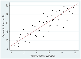
A fifth-year PhD candidate paid a visit to 221ß Baker Street. Sherlock decided to help him pass his final defence and began to give him a crash course on statistics—but the contents eventually cover many fundamental issues of statistics. For starters, Sherlock gave a test about simple regression. The fifth-year PhD student answered pretty well (from our eyes). Now, how will our friend Sherlock react? Let’s look through a crack in the door. Oh, the student drew the simplest possible regression model in the last episode.

“Oh, nice work. Now, that’s more like it. You must be a statistician! So, using your beautiful graph, will you kindly explain the four assumptions applied to the regression?”

Figure 1 Example of simple regression model from the last episode.¹

The student begins to talk, “First, ‘L’ means linear relation between the x-value and y-value of observations. As we can see on the board, the larger the x-value, the higher the y-value of an observation. Then, ‘I,’ um… this means independence… Ah, each dot, that is, each observation, is independent from the others!” The student begins to speak faster, looking as if he is excited.

“Now ‘N.’ It’s normal: If we draw a histogram or kernel density plot with the value of the dependent variable, it must be distributed normally or at least similarly. Finally, ‘E’ equals variance. Sorry, I don’t really know what that means.”

Sherlock sighs deeply and says, “Well, quite honestly, your level of understanding on the regression assumptions is world class.”

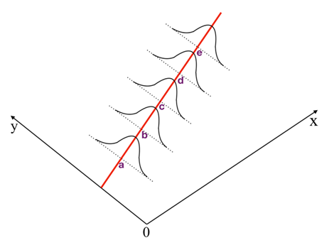
John walks to the whiteboard and begins to erase everything on it. He must feel the impending death of the virgin spirit… too virgin as a person facing his final defense. “Good luck and rest in peace,” John tells the student, patting him on his shoulder. Now it’s Sherlock’s time. He stands and draws a graph. It looks like the student’s but, clearly, there are more components. Most of all, it is three-dimensional.

Figure 2 A three-dimensional presentation of a linear regression.²

Sherlock begins to explain. “Yes, you use the mnemonic ‘LINE’ well, and indeed ‘L’ for linear relation is quite true. But the other three have issues. First is the independence assumption. Independent is not what you mean; it is conditionally independent. That is, if you fit the linear model like what’s on the whiteboard, the so-called residuals ̶ the difference between the fitted value (a-e) ̶ are independent. Otherwise, if the independence means an unconditional relationship, there cannot be a linear regression. What line can we draw? The point is that the line is controlling for disturbances of seemingly random locations of observation on the plane. Then, the rest are easy. Again, focus only on five points, a-e; observations lie around them or, more precisely, perpendicular to the x line. The observations tend to spread as in a normal distribution. Also, for every fitted point, there is the ‘same width normal distribution.’ This is what you call normality and equal variance mean.”

Sherlock returns to his normal cold character and says, “Get out! Come back the day after tomorrow. Homework is to explain the residual plot using the above four assumptions.

To be continued…

References

Jeong HJ. 221β Baker street, episode 2: The blind regressor-Part 1. Biom Biostat Int J. 2018;7(2): p. 123.
Rabe-Hesketh S, A Skrondal. Multilevel and Longitudinal Modeling Using Stata. 3rd edn. Vol. 1, College Station, TX: Stata Press; 2012.
Carson NR, CD Heat. Psychology the Science of Behavior. Ontario, CA: Pearson Education; 2010.