Research Article Volume 6 Issue 3
Size-biased poisson-garima distribution with applications
Rama Shanker,
shankerrama2009@gmail.com
Kamlesh Kumar Shukla
Department of Statistics, Eritrea Institute of Technology, Eritrea
Correspondence: Rama Shanker, Department of Statistics, Eritrea Institute of Technology, Asmara, Eritrea
Received: August 23, 2017 | Published: August 28, 2017
Citation: Shanker R, Shukla KK. Size-biased poisson-garima distribution with applications. Biom Biostat Int J. 2017;6(3):335-340. DOI: 10.15406/bbij.2017.06.00167
Download PDF
Abstract
In this paper, a size-biased Poisson-Garima distribution (SBPGD) has been obtained by size-biasing the Poisson-Garima distribution (PGD) introduced by Shanker (2017). The moments about origin and moments about mean have been obtained and hence expressions for coefficient of variation (C.V.), skewness and Kurtosis have been obtained. The estimation of its parameter using the method of moment and the method of maximum likelihood estimation has been discussed. The goodness of fit of SBPGD has been discussed for two real data sets using maximum likelihood estimate and the fit shows quite satisfactory over size-biased Poisson distribution (SBPD) and size-biased Poisson-Lindley distribution (SBPLD).
Keywords: garima distribution, poisson-garima distribution, size-biasing, moments, estimation of parameter, goodness of fit
Introduction
Shanker1 has obtained Poisson-Garima distribution (PGD) for modeling count data having probability mass function (p.m.f.)
(1.1)
The first four moments about origin and the variance of PGD obtained by Shanker1 are as follows:
,
,
, and
The detailed discussion about its properties, estimation of parameter, and applications has been discussed by Shanker1 and it has been shown that it is better than Poisson and Poisson-Lindley distributions for modeling count data in various fields of knowledge. The PGD arises from the Poisson distribution when its parameter
follows Garima distribution introduced by Shanker2 having probability density function (p.d.f.)
(1.2)
Size-biased distributions arise in practice when observations from a sample having probability proportional to some measure of unit size. Fisher3 firstly introduced these distributions to model ascertainment biases which were later formalized by Rao4 in a unifying theory. Size-biased observations occur in many research areas and its fields of applications includes medical science, sociology, psychology, ecology, geological sciences etc. The applications of size-biased distribution theory in fitting distributions of diameter at breast height (DBH) data arising from horizontal point sampling (HPS) has been discussed by Van Deusen.5 Further, Lappi and Bailey6 have applied size-biased distributions to analyze HPS diameter increment data. The statistical applications of size-biased distributions to the analysis of data relating to human population and ecology can be found in Patil and Rao.7,8 Some of the recent results on size-biased distributions pertaining to parameter estimation in forestry with special emphasis on Weibull family have been discussed by Gove.9 Ducey and Gove10 discussed size-biased distributions in the generalized beta distribution family, with applications to forestry.
Let a random variable
has the original probability distribution
, then a simple size-biased distribution is given by its probability function
(1.3)
Where
is the mean of the original probability distribution.
In the present paper, a size-biased Poisson-Garima distribution (SBPGD) has been proposed. It s raw and central moments and central moments based properties including coefficient of variation, skewness, kurtosis and index of dispersion have been obtained and discussed. Some of its statistical properties have been discussed. The method of moment and the method of maximum likelihood estimation have been discussed for estimating the parameter of SBPGD. The goodness of fit of SBPGD has also been presented.
Size-biased poisson-garima distribution
Using (1.1) and (1.3), the p.m.f. of the size-biased Poisson-Garima distribution (SBPGD) with parameter
can be obtained as
(2.1)
where
is the mean of the PGD (1.1).
The SBPGD can also be obtained from the size-biased Poisson distribution (SPBD) with p.m.f.
(2.2)
when its parameter
follows size-biased Garima distribution (SBGD) with p.d.f.
(2.3)
Thus the p.m.f of SBPGD can be obtained as
(2.4)
which is the p.m.f of SBPGD with parameter
.
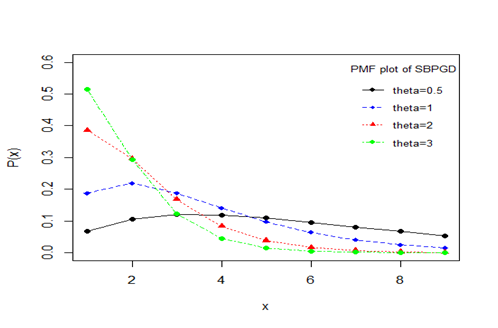
Graphs of SBPGD for varying values of parameter
are shown in figure 1. It is obvious from the graphs of SBPGD that as the value of parameter
increases, the initially the graphs shift upward and decreases fast for increasing values of
. Also the graphs become convex for values of
.

Figure 1 Graphs of SBPGD for varying values of parameter
.
It would be recalled that the p.m.f of size-biased Poisson-Lindley distribution (SBPLD) given by
(1.7)
has been introduced by Ghitany and Mutairi,11 which is a size-biased version of Poisson-Lindley distribution (PLD) introduced by Sankaran.12 Ghitany and Mutairi11 have discussed its various mathematical and statistical properties, estimation of the parameter using maximum likelihood estimation and the method of moments, and goodness of fit. Shanker et al.,13 has detailed study on the applications of size-biased Poisson-Lindley distribution (SBPLD) for modeling data on thunderstorms and observed that in most data sets, SBPLD gives better fit than size-biased Poisson distribution (SBPD).
Moments and moments based measures
Using (2.4), the
th factorial moment about origin of the SBPGD (2.1) can be obtained as
Taking
, we get
(3.1)
Substituting
, the first four factorial moments about origin can be obtained and using the relationship between factorial moments about origin and moments about origin, the first four moments about origin of SBPGD can be obtained as
Using the relationship between moments about mean and the moments about origin, the moments about mean of the SBPGD are thus obtained as
The coefficient of variation
, coefficient of Skewness
, coefficient of Kurtosis
and the index of dispersion
of the SBPGD are thus obtained as
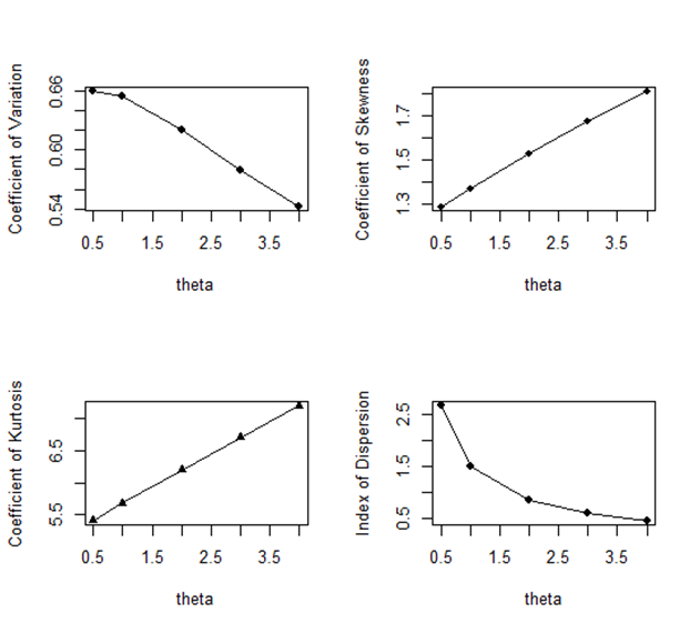
Graphs of coefficient of variation, coefficient of skewness, coefficient of kurtosis and index of dispersion of SBPGD for varying values of parameter
are shown in figure 2. It is obvious from the graphs that C.V and the index of dispersion are monotonically decreasing while the coefficient of skewness and coefficient of kurtosis are decreasing for increasing value of the parameter
.

Figure 2 Graphs of coefficient of variation, coefficient of skewness, coefficient of kurtosis and index of dispersion of SBPGD for varying values of parameter
.
The condition under which SBPGD and SBPLD are over-dispersed, equi-dispersed or under-dispersed are presented in table 1.
Distributions |
Over-dispersion
|
Equi-dispersion
|
Under-dispersion
|
SBPGD |
|
|
|
SBPLD |
|
|
|
Table 1 Over-dispersion, equi-dispersion and under-dispersion of SBPGD and SBPLD
Statistical properties of SBPGD
Unimodality and increasing failure rate
Since
is a deceasing function of
,
is log-concave. Therefore, SBPGD is unimodal, has an increasing failure rate (IFR), and hence increasing failure rate average (IFRA). It is new better than used in expectation (NBUE) and has decreasing mean residual life (DMRL). Detailed discussion about definitions and interrelationships between these aging concepts are available in Barlow and Proschan.14
Generating functions
Probability Generating Function: The probability generating function of the SBPGD (2.1) can be obtained as
Moment generating function: The moment generating function of the SBPGD (2.1) can be given by
Estimation of parameter
Method of moment estimate (MOME): Let
be a random sample of size
from the SBPGD (2.1). Equating the population to the corresponding sample mean, the MOME
of
of SBPGD (2.1) can be obtained as
where
is the sample mean.
Maximum likelihood estimate (MLE): Let
be a random sample of size
from the SBPGD (2.1) and let
be the observed frequency in the sample corresponding to
such that
, where
is the largest observed value having non-zero frequency. The likelihood function
of the SBPGD (2.1) is given by
The log likelihood function is obtained as
The first derivative of the log likelihood function is given by
where
is the sample mean.
The maximum likelihood estimate (MLE),
of
is the solution of the equation
and is given by the solution of the non-linear equation
This non-linear equation can be solved by any numerical iteration methods such as Newton- Raphson method, Bisection method, Regula –Falsi method etc. note that in this paper, we have solved above equation using Newton-Raphson method where the initial value of
is the value given by the method of moment estimate.
Data analysis
In this section, we fit SBPGD using maximum likelihood estimate to test its goodness of fit over SBPD and SBPLD. The first data-set is the immunogold assay data of Cullen et al.,15 regarding the distribution of number of counts of sites with particles from immunogold assay data, the second data-set is the number of European red mites on apple leaves, reported by Garman16 (Tables 2&3).
It is obvious from above tables that SBPGD gives better fit than both SBPD and SBPLD
No. of sites with particles |
Observed frequency |
Expected frequency |
SBPD |
SBPLD |
SBPGD |
1
2
3
4
5 |
122
50
18
4
4 |
111.3
64.1
|
119.0
53.8
18.0
|
119.1
53.7
18.0
|
Total |
198 |
198.0 |
198.0 |
198.0 |
ML estimate |
|
|
|
|
|
|
4.642 |
0.51 |
0.40 |
d.f. |
|
1 |
2 |
2 |
p-value |
|
0.031 |
0.7749 |
0.8187 |
Table 2 Distribution of number of counts of sites with particles from immunogold data
Number of European red mites |
Observed frequency |
Expected frequency |
SBPD |
SBPLD |
SBPGD |
1 |
38 |
28.7 |
31.7 |
31.9 |
2 |
17 |
25.7 |
23.9 |
23.8 |
3 |
10 |
15.3 |
13.2 |
13.1 |
4
5
6
7
8 |
9
3
2
1
0 |
|
|
|
Total |
80 |
80.0 |
80.0 |
80.0 |
ML estimate |
|
|
|
|
|
|
9.827 |
5.30 |
5.11 |
d.f. |
|
2 |
2 |
2 |
P-value |
|
0.0073 |
0.0706 |
0.0777 |
Table 3 Number of European red mites on apple leaves, reported by Garman (1923)
Acknowledgements
None.
Conflicts of interest
None.
References
- Shanker R. The Discrete Poisson‒Garima Distribution. Biom Biostat Int J. 2017;5(2):00127.
- Shanker R. Garima Distribution and its Application to Model Behavioral Science Data. Biom Biostat Int J. 2016;4(7):00116.
- Fisher RA. The effects of methods of ascertainment upon the estimation of frequencies. Ann Eugenics. 1934;6(1):13‒25.
- Rao CR. On discrete distributions arising out of methods of ascertainment In: Patil GP (Ed.), Classical and Contagious Discrete Distributions. Statistical Publishing Society, Calcutta. 1965;pp. 320‒332.
- Van Deusen PC. Fitting assumed distributions to horizontal point sample diameters. For Sci. 1986;32(1):146‒148.
- Lappi J, Bailey RL. Estimation of diameter increment function or other tree relations using angle‒count samples. Forest science. 1987;33:725‒739.
- Patil GP, Rao CR. The Weighted distributions: A survey and their applications. In applications of Statistics (Ed P.R. Krishnaiah, North Holland Publications Co., Amsterdam. 1977;pp. 383‒405.
- Patil GP, Rao CR. Weighted distributions and size‒biased sampling with applications to wild‒life populations and human families. Biometrics. 1978;34(2):179‒189.
- Gove JH. Estimation and applications of size‒biased distributions in forestry. In Modeling Forest Systems. In: Amaro A, et al. (Eds), CABI Publishing, USA. 2003;pp. 201‒212.
- Ducey MJ, Gove JH. Size‒biased distributions in the generalized beta distribution family, with applications to forestry. Forestry‒ An International Journal of Forest Research. 2015;88:143‒151.
- Ghitany ME, Al‒Mutairi DK. Size‒biased Poisson‒Lindley distribution and Its Applications. Metron ‒ International Journal of Statistics LXVI. 2008;(3):299‒311.
- Sankaran M. The discrete Poisson‒Lindley distribution. Biometrics. 1970;26(1):145‒149.
- Shanker R, Hagos F, Abrehe Y. On Size –Biased Poisson‒Lindley Distribution and Its Applications to Model Thunderstorms. American Journal of Mathematics and Statistics. 2015;5(6):354‒360.
- Barlow RE, Proschan F. Statistical Theory of Reliability and Life Testing, Silver Spring, MD. 1981.
- Cullen MJ, Walsh J, Nicholson LV, et al. Ultrastructural localization of dystrophin in human muscle by using gold immunolabelling. Proc R Soc Lond B Biol Sci. 240(1297):197‒210.
- Garman P. The European red mites in Connecticut apple orchards. Connecticut Agri Exper Station Bull. 1923;252:103‒125.
- Lindley DV. Fiducial distributions and Bayes theorem. Journal of the Royal Statistical Society. 1958;20(1):102‒107.

©2017 Shanker, et al. This is an open access article distributed under the terms of the,
which
permits unrestricted use, distribution, and build upon your work non-commercially.


