Accordingly to FDA draft guidance (2010), adaptive randomization (e.g. response-adaptive (RA) randomization) has become popular in clinical research because of its flexibility and efficiency, which also have the advantage of assigning fewer patients to inferior treatment arms. The RA design based on binary outcome is commonly used in clinical trial where “success” is defined as the desired (or undesired) event occurring within (or beyond) a clinical relevant time. As patients entering into trial sequentially, only part of patients have sufficient follow-up during interim analysis. This results in a loss of information as it is unclear how patients without sufficient follow-up should be handled. Alternatively, adaptive design for survival trial was proposed for this type of trial. However, most of current practice assumes the event times following a pre-specified parametric distribution. We adopt a nonparametric model of survival outcome which is robust to model of event time distribution, and then apply it to response-adaptive design. The operating characteristics of the proposed design along with parametric design are compared by simulation studies, including their robustness properties with respect to model misspecifications.

Keywords: adaptive design, clinical trials, bayesian adaptive design, survival analysis

Response-adaptive (RA) randomization scheme has become popular in clinical research because of its flexibility and efficiency. Based on the accruing history of patients’ responses to treatment, the RA randomization scheme adjusts the future allocation probabilities, thereby allowing more patients to be assigned to the superior treatment as the trial progresses. As a result, RA randomization can offer significant ethical and cost advantages over equal randomization.

The RA design based on binary outcome is commonly used in clinical trial where “success” is defined as the desired (or undesired) event occurring within (or beyond) a clinical relevant time. As patients entering into trial sequentially, only part of patients have sufficient follow-up during interim analysis. This results in a loss of information as it is unclear how patients without sufficient follow-up should be handled. Alternatively, adaptive design for survival trial was proposed for this type of trial.

However, most of current practice assumes the event times following a pre-specified parametric distribution. We adopt a nonparametric model of survival outcome which is robust to model of event time distribution, and then apply it to response-adaptive design. The operating characteristics of the proposed design along with parametric design are compared by simulation studies, including their robustness properties with respect to model misspecifications.

A nonparametric survival model

Patients are enrolled in sequential groups of size {Nj }, j =1, . . . , J , where Nj is the sample size of the sequential group j . Typically, before conducting the trial, researchers have little prior information regarding the superiority of the treatment arms. Therefore, initially, for the first j’ groups, e.g. j’=1, patients are allocated to K treatment arms with an equal probability 1/K. As patients accurate, the number of current patients increased. Let Ti be the event time for patient i and τ be the clinical relevant time where $\theta =\mathrm{Pr}(T>\tau )$ is the event of interest. For example, a trial is conducted to assess the progression-free survival probability at 9 months. During the trial, the number of current patients increased as patients accurate. Let N(t) denote the current number of patients who have been accrued and treated at a given calendar time t during the trial. Without censoring, $\theta$ can be modeled by binomial model where the likelihood function evaluated at time t is

$\text{L}\left(data\text{|θ}\right)={\Pi }_{i=1}^{N(t)}{\text{θ}}^{\text{I}({\text{T}}_{\text{i}}>\tau )}{\left(1-\text{θ}\right)}^{\text{I}\left({\text{T}}_{\text{i}}\le \text{τ}\right)}$  (1)

However, censoring is not avoidable in clinical practice. As patients enter into the trial sequentially, the follow-up time for certain patients may less than τ when we evaluate $\theta$  at any calendar time t. Other reason for censoring, including, but not limited to, patient drop out, failure to measure the outcome of interest, and so on. If we ignore the censoring, substantial information will be lost. Cheung & Chappell¹ introduced a simple model for dose-finding trial. Later, Cheung & Thall² adopted this model to continuous monitoring for phase II clinical trials. With censoring, the likelihood function (1) can be rewritten as

$L\left(data|\theta \right)={\Pi }_{i=1}^{N(t)}\mathrm{Pr}\mathrm{Pr}{\left\{T_i\pounds \min \min \left(x_i,\tau \right)\right\}}^{Y\left(x_i\right)}\mathrm{Pr}{\{T_i>\min \min \left(x_i,\tau \right)\}}^{1-Y\left(x_i\right)}$  (2)

Where $x_i=\min \left(c_i,t_i\right)$ is the observed event time, c_i is the censoring time, and $Y\left(x_i\right)=I\{T_i\le \min \min \left(x_i,\tau \right)\}$ is the censoring indicates function.

Furthermore, the parameter $\theta$ will be plug into the likelihood function through probability transformation,

$\mathrm{Pr}\mathrm{Pr}\left({\text{T}}_{\text{i}}\le \text{t}\right)=\mathrm{Pr}\mathrm{Pr}\left({\text{T}}_{\text{i}}\le \text{t},{\text{T}}_{\text{i}}\le \text{τ}\right)+\mathrm{Pr}\mathrm{Pr}\left({\text{T}}_{\text{i}}\le \text{t},{\text{T}}_{\text{i}}>\tau \right)$

$=\mathrm{Pr}\mathrm{Pr}\left({\text{T}}_{\text{i}}\le \text{t}|{\text{T}}_{\text{i}}\le \text{τ}\right)\mathrm{Pr}\mathrm{Pr}\left({\text{T}}_{\text{i}}\le \text{τ}\right)\text{f}\left({\text{T}}_{\text{i}}\le \text{τ}\right)+\mathrm{Pr}\mathrm{Pr}\left({\text{T}}_{\text{i}}\le \text{t}|{\text{T}}_{\text{i}}\rangle \tau \right)$ $Pr()$ $=w\left(t\right)\left(1-\theta \right)$  (3)

Where $w\left(t\right)=\{\begin{array}{c}\mathrm{Pr}(T_i\le t|T_i\le \tau )\\ 1\end{array}\begin{array}{c},t\le \tau \\ t>\tau \end{array}$ , is a weight function

Finally, we can obtain a working likelihood with unbiased estimation of w(t).

$\text{L}\left(\text{data|θ}\right)={\displaystyle \prod }_{\text{i}=1}^{\text{N}\left(\text{t}\right)}\tilde{w}\left({\text{x}}_{\text{i}}\right){\left(1-\text{θ}\right)}^{\text{Y}\left({\text{x}}_{\text{i}}\right)}{\left\{1-\tilde{w}\left({\text{x}}_{\text{i}}\right)\left(1-\text{θ}\right)\right\}}^{1-\text{Y}\left({\text{x}}_{\text{i}}\right)}$ (4)

Theorem: if $\tilde{w}\left({\text{x}}_{\text{i}}\right)$ converges almost surely to $\tilde{w}\left({\text{x}}_{\text{i}}\right)$  for all I as $N\left(t\right)\to \infty$ , then $\widehat{\theta }=\arg \max L(\text{data}|\theta )$ is strongly consistent for true survival probability $\theta$ .

Cheung & Chappell [1] assumed the nuisance parameter $\tilde{w}\left({\text{x}}_{\text{i}}\right)$  as a linear function $\tilde{w}\left({\text{x}}_{\text{i}}\right)=x_i/\tau$ . Ji & Bekele³ shows that these estimated weights are based on strong assumption of linearity and independence; it may leads to biased results when the assumptions are violated. We propose to estimate $\tilde{w}\left({\text{x}}_{\text{i}}\right)$  with KM estimation, where

$\tilde{w}\left({\text{x}}_{\text{i}}\right)=\frac{1-\tilde{S}\left({\text{x}}_{\text{i}}\right)}{1-\tilde{S}\left(\text{τ}\right)}$

It’s easy to show that $\tilde{w}\left(x_i\right)$  is a unbiased estimation of $\left(x_i\right)$ .

Adaptive randomization

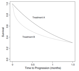
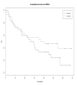
Under model (4), the survival probability evaluated at time $\tau$ , is used as a conventional measure of treatment efficacy. However, such a survival probability at $\tau$  ignores the entire path of survival curve. While, particular interest in a clinical trial is the estimation of the difference between survival probability for the treatment groups at several points in time. As shown in Figure 1, the survival curve under treatment B declines faster than that under treatment A, although both treatments have the same survival probability at $\tau$ . In the renal cancer trial, this indicates that patients under treatment B would experience disease progression much faster than those under treatment A. Because delayed disease progression typically leads to a better quality of life, treatment A would be preferred in this situation.^4,5 Another example is showed in Figure 2. The survival curves are almost identical between two treatments before time 20. If we compare the survival probability between two treatments at the time before 20, the treatment effect is inconclusive. To provide a comprehensive measure of efficacy by accounting for the shape of the survival curve, we propose to evaluate survival probability at several points in time. Let $\theta kj$  be the survival probability at time $\tau j$  for treatment k where $j=1,\dots ,J$ . The treatment allocation probability for treatment k is defined as,

${\text{π}}_{\text{k}}={\displaystyle \sum }_{\text{j}=1}^{\text{J}}{\text{w}}_{\text{j}}\text{Pr}({\text{θ}}_{\text{kj}}=\text{max}\left\{{\text{θ}}_{\text{lj}},1\le \text{l}\le \text{J}\right\}|\text{data})$

Where wj is the prespecified weight. Currently, we use equal weight with $wj=1/J$ .

Figure 1 Survival curves of the time to disease progression, where the two survival curves have the same survival probability at the follow-up time $\tau =1.5$ months, but different areas under the survival curves until $\tau$ .

Figure 2 Survival curves of the time to disease progression, where the two survival curves have the same survival probability before week 20, but gradually show difference as time increase.

During the trial, we continuously monitor posterior probability of ${\pi }_k$ . When the efficacy of ${\pi }_k$  is lower than the prespecified lower limit pl, then the treatment arm k will be terminated early due to futility. When ${\pi }_k$  is higher than pu, the treatment arm k will be selected as promising treatment. In practice, the values of pl and pu are chosen by simulation studies in order to achieve desirable operating characteristics for the trial.

We simulate a single arm trial where the event times follow weibull distribution with $\alpha =2$  and $\lambda =50$ . And, patients enter into the trial sequentially with accrual rate of one per week. At week 50, we stop enrol the patients and continue to follow the trial for additional 30 weeks. The parameter of interesting is $\theta =Pr\left(T>40\right)$ .

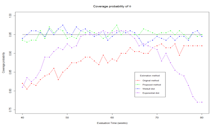
The purpose of this simulation study is to compare the performance of estimation with different methods and to show whether the estimation at different trial monitoring time is consistent. Four estimation method will be evaluated, including proposed method, true parametric method (weibull distribution), misspecified parametric method (exponential distribution), and original method $(\tilde{w}\left(x_i\right)=x_i/\tau )$ . Trial monitoring starts at time 40 and continue until the end of study. Figure 3 shows the estimated θ at different monitoring time. The results show that the true parametric method and proposed method can provide unbiased estimation over monitoring time while the original method and misspecified parametric method give large bias. Its worth to note that the original method gives small bias at the end of trial because the number of censored observed decreased as follow-up time increase. In Figure 4, we present the coverage probability along the monitoring times. The figure shows that the proposed method and true parametric method provide constant coverage probability over the monitoring time which is close to the nominal value of 95%. While the original method and misspecified parametric method provides low coverage probability.

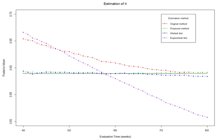
Figure 3 Estimated $\theta$  with different method.

Figure 4 Coverage probability of $\theta$  with different method.

Adaptive randomization

We conducted simulations to evaluate the performance of the proposed adaptive randomization design under various clinical scenarios (1000 simulations per scenario). For the simulations, we set the accrual rate to two patients per week. The maximum number of patients is 120. After the initial 60 weeks of enrollment time, there is an additional follow-up period of 40 weeks. The event times are simulated from weibull distribution with $\alpha =1$  in scenario I and $\alpha =0.5$ in scenario II. We assigned the first 30 patients equally to two arms (A or B) and started using the adaptive randomization at the 31^st patient. The proposed design will be compared with the following designs: parametric design (exponential distribution) and original design $(\tilde{w}\left(x_i\right)=x_i/\tau )$ .

Table 1 shows the simulation results where event times simulated from exponential distribution. For each design, we list the average number of patients (with percentage of total patients in the trial) assigned to each treatment arm, and the chance of a treatment being selected as promising. Comparing the proposed design and parametric designs, the proposed design provides comparable operational characteristic where both design assign more patients to more promising treatment (69% for proposed design and 70.3% for parametric design) and both design provide the sample level of power (0.978 for proposed design and 0.979 for parametric design). While the original design provides lower power than then proposed design and parametric design.

Table 2 shows simulation results for scenario II. In the presence of event time distribution misspecification, the parametric design provides lower power than proposed design (0.836 vs 0.647). And, the proposed design assigns more patients to more promising treatment. Once again, the original design has lower power than the other two designs.

We have developed a Bayesian response-adaptive randomization design for survival trial. A nonparametric survival model is applied to estimate the survival probability at a clinical relevant time. The proposed design provides comparable operational characteristics as true parametric design. Whereas, the proposed design perform better than parametric design when the event time distribution is misspecified. The proposed design can be extended to Response-Adaptive Covariate-Adjusted Randomization (RACA) design when we need to control important prognostics among treatment arms. The benefits of adaptive randomization for survival trial depend on the distributions of event times and patient accrual rate as well as on the particular adaptive design under consideration. If there are short-term response quickly available and can predicting the long-term survival, we can used those short-term response to “speed up” adaptive randomization for survival trial.

None.

Author declares that there are no conflicts of interest.

1. Cheung YK, Chappell R.  Sequential designs for phase I clinical trials with late-onset toxicities. Biometrics. 2000;56(4):1177–1182.
2. Cheung YK, Thall PF. Monitoring the rates of composite events with censored data in phase II clinical trials. Biometrics. 2002;58(1):89–97.
3. Ji Y, Bekele BN. Adaptive randomization for multiarm comparative clinical trials based on joint efficacy/toxicity outcomes. Biometrics. 2009;65(3):876–884.
4. Case LD, Morgan TM. Design of phase II cancer trials evaluating survival probabilities. BMC Med Res Methodol. 2003;3(1):6.
5. Huang X, Ning J, Li Y, et al. Using short-term response information to facilitate adaptive randomization for survival clinical trials. Stat in Medicine. 2009;28(12):1680–1689.

References

Creative Commons Attribution License
©2016 Lin, et al. This is an open access article distributed under the terms of the, which permits unrestricted use, distribution, and build upon your work non-commercially.