Submit manuscript...
eISSN: 2378-315X

Biometrics & Biostatistics International Journal

Research Article Volume 1 Issue 3

Relative accuracy of the screening tests when absolute determination of the disease status is not feasible

Keter K Alfred,1 Otieno R Argwings2

1Academic Model Providing Access to Healthcare (AMPATH), Kenya
2Department of Mathematics and Computer Science, University of Eldoret, Kenya

Correspondence: K Alfred, Academic Model Providing Access to Healthcare (AMPATH), Eldoret, Kenya, Tel 254 722 792 928

Received: November 05, 2014 | Published: December 4, 2014

Citation: Alfred KK, Josphat KK, Alfred K, et al. Relative accuracy of the screening tests when absolute determination of the disease status is not feasible. Biom Biostat Int J. 2014;1(3):85-90. DOI: 10.15406/bbij.2014.01.00016

Download PDF

Abstract

Comparison of the accuracy of a new screening test to that of the standard one can be implemented by administering both screening tests to a group of asymptomatic subjects for which the disease status can be determined using a gold standard (GS) test. Nevertheless, the GS test may be too costly or too invasive hence unethical to administer to all the study subjects, including those who screen negative on all the screening tests. When this is the case, relative accuracy of the two screening tests can be estimated when a randomized paired screen positive (RPSP) design is used to collect the data. However, this design contains cells with missing data, thus the likelihood function is not available. The objective of this study is to demonstrate a parsimonious way of estimating relative accuracy of the screening tests when the determination of the disease status of the subjects who screened negative on the new and the standard screening tests was not conducted due to ethical concerns.

Markov Chain Monte Carlo simulation technique is used to parsimoniously address the aforementioned shortcoming of the RPSP design when subjective approach to estimation is used. Multiple data imputation using Gibbs sampler is performed. Monte Carlo point and interval estimates of the missing data, measures of accuracy and the relative rates are computed when the tests are treated to be:

  1. Conditionally independent
  2. Dependent

The accuracy when the tests are dependent is higher than when the tests are conditionally independent. This is apparent from the narrower credible bounds and smaller standard errors of the true and false positive rates under this setting. Secondly, the estimates obtained under the two assumptions are better than when the missing data are ignored. Whether these differences were true or just due to chance warrant statistical investigation under different assumptions.

Keywords: conditional independence, dependence, gibbs sampling, markov chain monte carlo, subjective approach, credible bounds

Abbreviations

TPR, true positive rate; FPR, false positive rate; DP, detection probabilities; FP, false referral probabilities; MCMC, markov chain monte carlo simulation; rTPR, relative true positive rate; rFPR, relative false positive rate; MAR, missing at random

Introduction

Before a new test is approved for public health use its accuracy should be compared to that of the existing standard tests to determine whether the new test is superior to or at least as accurate as the available tests. This is achieved through the use of standard metrics used to compare the true positive rate (TPR) and the false positive rate (FPR) of two tests. This comparison is quantified using the relative performance or the relative accuracy of the tests used for detecting the disease.15 Screen positive designs administer the gold standard test to subjects with positive outcome on at least one of the screening tests. These designs are preferred if the diagnostic test is too costly or too invasive to be applied to all the study subjects.

It is unethical to administer a cancer-confirming biopsy to subjects who screen negative on both the new and the standard screening tests because the results already suggest a low probability of cancer.2,4 Therefore the biopsy data are missing with negative screening tests. This is what we end up with in screen positive designs. In this case disease detection probabilities (DP) and false referral probabilities (FP) are the key measures of accuracy that can be derived.4 These estimates will be biased because some subjects might have been missed by the screening test due to error. A way to mitigate this issue is to impute the missing data. Therefore the aim of this study is to demonstrate a parsimonious way of estimating relative accuracy of the screening tests when the determination of the disease status of the subjects who screened negative on the new and the standard screening tests was not conducted due to ethical concerns. Markov Chain Monte Carlo simulation (MCMC) technique was used to address the aforementioned shortcoming when subjective approach to estimation was adopted..6,7 Non-informative conjugate prior distributions were utilized.

Inferences about the performance of the screening tests are based on the estimates of relative true positive rate (rTPR) and relative false positive rate (rFPR). These rates are respectively obtained by taking the ratio of the point estimates of TPR and FPR of the new screening test to that of the standard screening test.14 In section 2 we give an outline of the methods that were used. The randomized paired screen positive design by4 is discussed in section 3. In this section we compute the measures of accuracy under the assumptions that the tests are

  1. Conditionally independent
  2. Dependent

The other assumptions were: data were observed with the RPSP design, the missing data were assumed to be missing at random (MAR), the TPR and the FPR of the standard screening test were assumed to be 0.5 and 0.02 respectively, and the rTPR and rFPR were assumed to be 1.5 and 1.25 respectively. In section 4 we provide the results while in section 5 we discuss, conclude and give recommendations.

Methods

Due to the missing data the likelihood function for the data was not available. Consequently the subjective as well as the classical approaches to estimation were intractable. Thus MCMC technique was adopted. When the new and the standard screening tests were assumed to be conditionally independent, the data followed binomial distribution thus the conjugate prior distribution was Beta distribution. When the new and the standard screening tests were assumed to dependent the data followed a multinomial distribution thus the conjugate prior distribution was Dirichlet distribution.8 Non-informative prior distributions were used. To get the posterior distributions data augmentation technique was utilized to circumvent the complexity resulting due to missing data. The missing data were assumed to be MAR. MCMC approach was applied and Monte Carlo point and interval estimates were reported. Multiple data imputation using Gibbs sampler was employed. The missing data and the measures of accuracy were imputed using the binomial and beta distributions respectively. Assuming we had the observed data resulting from the subjects who screened positive for at least one screening test under RPSP design, the simulation proceeded as follows: Initialize by estimating the parameter of interest from the posterior distribution of interest then draw a missing value from the posterior distribution of the missing data. Next draw a parameter of interest from the posterior distribution of interest again then the missing data from the posterior distribution of the missing data. This procedure was iterated 10000 times. One run of 10000 draws was implemented. Analysis of the chain was performed to establish the convergence.9,10 The sample size in our study was 45900 and the prevalence of the disease was assumed to be 1%.

Design and estimation

Randomized paired screen positive (RPSP) design

In RPSP design n subjects are randomized to first receive test X1 or test X2. The second screening test and the GS test are administered only if the first screening test was positive.4 Data from such a design are summarized in (Table 1).

The variables n j k l p MathType@MTEF@5@5@+=feaaguart1ev2aqatCvAUfeBSjuyZL2yd9gzLbvyNv2CaerbuLwBLnhiov2DGi1BTfMBaeXatLxBI9gBaerbd9wDYLwzYbItLDharqqtubsr4rNCHbGeaGqkY=xjYJH8sqFD0xXdHaVhbbf9v8qqaqFr0xc9pk0xbba9q8WqFfeaY=biLkVcLq=JHqpepeea0=as0Fb9pgeaYRXxe9vr0=vr0=vqpWqaaeaabiGaciaacaqabeaadaqaaqaaaOqaaiaad6gadaqhaaWcbaGaamOAaiaadUgacaWGSbaabaGaamiCaaaaaaa@3D1C@ and z j k l p MathType@MTEF@5@5@+=feaaguart1ev2aqatCvAUfeBSjuyZL2yd9gzLbvyNv2CaerbuLwBLnhiov2DGi1BTfMBaeXatLxBI9gBaerbd9wDYLwzYbItLDharqqtubsr4rNCHbGeaGqkY=xjYJH8sqFD0xXdHaVhbbf9v8qqaqFr0xc9pk0xbba9q8WqFfeaY=biLkVcLq=JHqpepeea0=as0Fb9pgeaYRXxe9vr0=vr0=vqpWqaaeaabiGaciaacaqabeaadaqaaqaaaOqaaiaadQhadaqhaaWcbaGaamOAaiaadUgacaWGSbaabaGaamiCaaaaaaa@3D28@ , p = 1 , 2 , j , k , l = 0 , 1 MathType@MTEF@5@5@+=feaaguart1ev2aqatCvAUfeBSjuyZL2yd9gzLbvyNv2CaerbuLwBLnhiov2DGi1BTfMBaeXatLxBI9gBaerbd9wDYLwzYbItLDharqqtubsr4rNCHbGeaGqkY=xjYJH8sqFD0xXdHaVhbbf9v8qqaqFr0xc9pk0xbba9q8WqFfeaY=biLkVcLq=JHqpepeea0=as0Fb9pgeaYRXxe9vr0=vr0=vqpWqaaeaabiGaciaacaqabeaadaqaaqaaaOqaaiaadchacqGH9aqpcaaIXaGaaiilaiaaykW7caaIYaGaaiilaiaaykW7caaMc8UaamOAaiaacYcacaWGRbGaaiilaiaadYgacqGH9aqpcaaIWaGaaiilaiaaykW7caaIXaaaaa@4A90@ , where
j = { 0 f o r a n e g a t i v e r e s u l t o n t e s t X 1 1 f o r a p o s i t i v e r e s u l t o n t e s t X 1 , k = { 0 f o r a n o n d i s e a s e d s u b j e c t 1 f o r a d i s e a s e d s u b j e c t MathType@MTEF@5@5@+=feaaguart1ev2aqatCvAUfeBSjuyZL2yd9gzLbvyNv2CaerbuLwBLnhiov2DGi1BTfMBaeXatLxBI9gBaerbd9wDYLwzYbItLDharqqtubsr4rNCHbGeaGqkY=xjYJH8sqFD0xXdHaVhbbf9v8qqaqFr0xc9pk0xbba9q8WqFfeaY=biLkVcLq=JHqpepeea0=as0Fb9pgeaYRXxe9vr0=vr0=vqpWqaaeaabiGaciaacaqabeaadaqaaqaaaOqaaiaadQgacqGH9aqpdaGabaqaauaabeqadiaaaeaacaaIWaaabaGaamOzaiaad+gacaWGYbGaaGPaVlaadggacaaMc8UaamOBaiaadwgacaWGNbGaamyyaiaadshacaWGPbGaamODaiaadwgacaaMc8UaamOCaiaadwgacaWGZbGaamyDaiaadYgacaWG0bGaaGPaVlaad+gacaWGUbGaaGPaVlaaykW7caWG0bGaamyzaiaadohacaWG0bGaaGPaVlaaykW7caWGybWaaSbaaSqaaiaaigdaaeqaaaGcbaaabaaabaGaaGymaaqaaiaadAgacaWGVbGaamOCaiaaykW7caWGHbGaaGPaVlaadchacaWGVbGaam4CaiaadMgacaWG0bGaamyAaiaadAhacaWGLbGaaGPaVlaadkhacaWGLbGaam4CaiaadwhacaWGSbGaamiDaiaaykW7caWGVbGaamOBaiaaykW7caaMc8UaamiDaiaadwgacaWGZbGaamiDaiaaykW7caaMc8UaamiwamaaBaaaleaacaaIXaaabeaaaaaakiaawUhaaiaaykW7caaMc8UaaiilaiaaykW7caaMc8UaaGPaVlaaykW7caWGRbGaeyypa0ZaaiqaaeaafaqabeWacaaabaGaaGimaaqaaiaadAgacaWGVbGaamOCaiaaykW7caWGHbGaaGPaVlaad6gacaWGVbGaamOBaiabgkHiTiaadsgacaWGPbGaam4CaiaadwgacaWGHbGaam4CaiaadwgacaWGKbGaaGPaVlaadohacaWG1bGaamOyaiaadQgacaWGLbGaam4yaiaadshaaeaaaeaaaeaacaaIXaaabaGaaGPaVlaadAgacaWGVbGaamOCaiaaykW7caWGHbGaaGPaVlaadsgacaWGPbGaam4CaiaadwgacaWGHbGaam4CaiaadwgacaWGKbGaaGPaVlaadohacaWG1bGaamOyaiaadQgacaWGLbGaam4yaiaadshacaaMc8UaaGPaVlaaykW7caaMc8UaaGPaVlaaykW7caaMc8UaaGPaVlaaykW7caaMc8UaaGPaVlaaykW7caaMc8UaaGPaVlaaykW7caaMc8oaaaGaay5Eaaaaaa@DFD8@ and

l = { 0 f o r a n e g a t i v e r e s u l t o n t e s t X 2 1 f o r a p o s i t i v e r e s u l t o n t e s t X 2 MathType@MTEF@5@5@+=feaaguart1ev2aqatCvAUfeBSjuyZL2yd9gzLbvyNv2CaerbuLwBLnhiov2DGi1BTfMBaeXatLxBI9gBaerbd9wDYLwzYbItLDharqqtubsr4rNCHbGeaGqkY=xjYJH8sqFD0xXdHaVhbbf9v8qqaqFr0xc9pk0xbba9q8WqFfeaY=biLkVcLq=JHqpepeea0=as0Fb9pgeaYRXxe9vr0=vr0=vqpWqaaeaabiGaciaacaqabeaadaqaaqaaaOqaaiaadYgacqGH9aqpdaGabaqaauaabeqadiaaaeaacaaIWaaabaGaamOzaiaad+gacaWGYbGaaGPaVlaadggacaaMc8UaamOBaiaadwgacaWGNbGaamyyaiaadshacaWGPbGaamODaiaadwgacaaMc8UaamOCaiaadwgacaWGZbGaamyDaiaadYgacaWG0bGaaGPaVlaad+gacaWGUbGaaGPaVlaaykW7caWG0bGaamyzaiaadohacaWG0bGaaGPaVlaaykW7caWGybWaaSbaaSqaaiaaikdaaeqaaaGcbaaabaaabaGaaGymaaqaaiaadAgacaWGVbGaamOCaiaaykW7caWGHbGaaGPaVlaadchacaWGVbGaam4CaiaadMgacaWG0bGaamyAaiaadAhacaWGLbGaaGPaVlaaykW7caWGYbGaamyzaiaadohacaWG1bGaamiBaiaadshacaaMc8Uaam4Baiaad6gacaaMc8UaaGPaVlaadshacaWGLbGaam4CaiaadshacaaMc8UaaGPaVlaadIfadaWgaaWcbaGaaGOmaaqabaaaaaGccaGL7baaaaa@8827@

denote the observed and the missing data, respectively, while the cells with “ ? MathType@MTEF@5@5@+=feaaguart1ev2aqatCvAUfeBSjuyZL2yd9gzLbvyNv2CaerbuLwBLnhiov2DGi1BTfMBaeXatLxBI9gBaerbd9wDYLwzYbItLDharqqtubsr4rNCHbGeaGqkY=xjYJH8sqFD0xXdHaVhbbf9v8qqaqFr0xc9pk0xbba9q8WqFfeaY=biLkVcLq=JHqpepeea0=as0Fb9pgeaYRXxe9vr0=vr0=vqpWqaaeaabiGaciaacaqabeaadaqaaqaaaOqaaiaac+dacqGHIaYTaaa@3A7F@ ” denote the unknown marginal totals. The superscripts denote the test that the subjects were first randomized to receive. Test X1 is the standard test while test X2 is the new test.

Measures of accuracy when the tests are assumed to be conditionally independent

The total number of subjects with the disease and without the disease in the design is fixed. Further, the row totals are fixed and the column totals are random. Thus binomial sampling model was appropriate for each test. Assume that the n 1 MathType@MTEF@5@5@+=feaaguart1ev2aaatCvAUfeBSjuyZL2yd9gzLbvyNv2CaerbuLwBLnhiov2DGi1BTfMBaeXatLxBI9gBaerbd9wDYLwzYbItLDharqqtubsr4rNCHbGeaGqk0Jf9crFfpeea0xh9v8qiW7rqqrFfpeea0xe9Lq=Jc9vqaqpepm0xbba9pwe9Q8fs0=yqaqpepae9pg0FirpepeKkFr0xfr=xfr=xb9adbaqaaeGaciGaaiaabeqaamaabaabaaGcbaGaamOBamaaBaaaleaacqGHIaYTcaaMc8UaaGymaiaaykW7cqGHIaYTaeqaaaaa@3FFF@ is equal to the actual sample size11 determined and n 0 MathType@MTEF@5@5@+=feaaguart1ev2aaatCvAUfeBSjuyZL2yd9gzLbvyNv2CaerbuLwBLnhiov2DGi1BTfMBaeXatLxBI9gBaerbd9wDYLwzYbItLDharqqtubsr4rNCHbGeaGqk0Jf9crFfpeea0xh9v8qiW7rqqrFfpeea0xe9Lq=Jc9vqaqpepm0xbba9pwe9Q8fs0=yqaqpepae9pg0FirpepeKkFr0xfr=xfr=xb9adbaqaaeGaciGaaiaabeqaamaabaabaaGcbaGaamOBamaaBaaaleaacqGHIaYTcaaMc8UaaGimaiabgkci3cqabaaaaa@3E73@ is equal to ( 1 ψ ψ ) n 1 MathType@MTEF@5@5@+=feaaguart1ev2aaatCvAUfeBSjuyZL2yd9gzLbvyNv2CaerbuLwBLnhiov2DGi1BTfMBaeXatLxBI9gBaerbd9wDYLwzYbItLDharqqtubsr4rNCHbGeaGqk0Jf9crFfpeea0xh9v8qiW7rqqrFfpeea0xe9Lq=Jc9vqaqpepm0xbba9pwe9Q8fs0=yqaqpepae9pg0FirpepeKkFr0xfr=xfr=xb9adbaqaaeGaciGaaiaabeqaamaabaabaaGcbaWaaeWaaeaadaWcbaWcbaGaaGymaiabgkHiTiabeI8a5bqaaiabeI8a5baaaOGaayjkaiaawMcaaiaad6gadaWgaaWcbaGaeyOiGCRaaGPaVlaaigdacaaMc8UaeyOiGClabeaaaaa@46F2@ where ψ MathType@MTEF@5@5@+=feaaguart1ev2aqatCvAUfeBSjuyZL2yd9gzLbvyNv2CaerbuLwBLnhiov2DGi1BTfMBaeXatLxBI9gBaerbd9wDYLwzYbItLDharqqtubsr4rNCHbGeaGqk0Jf9crFfpeea0xh9v8qiW7rqqrFfpeea0xe9Lq=Jc9vqaqpepm0xbba9pwe9Q8fs0=yqaqpepae9pg0FirpepeKkFr0xfr=xfr=xb9adbaqaaeGaciGaaiaabeqaamaabaabaaGcbaGaeqiYdKhaaa@39D4@ is the prevalence of the disease in the population. The marginal totals of the tests can be approximated based on the assumed TPRs or FPRs of the tests. (Table 2) summarizes the data from the RPSP design under the assumption that the tests are conditionally independent. (Table 2) is similar to the unpaired screen positive (USP) design.14

Where
n 111 = n 111 1 + n 111 2 + n 110 1 + z 110 2 , n 110 = n 011 2 + z 011 1 + z 010 2 , n 011 = n 111 1 + n 111 2 + n 011 2 + z 011 1 MathType@MTEF@5@5@+=feaaguart1ev2aaatCvAUfeBSjuyZL2yd9gzLbvyNv2CaerbuLwBLnhiov2DGi1BTfMBaeXatLxBI9gBaerbd9wDYLwzYbItLDharqqtubsr4rNCHbGeaGqk0Jf9crFfpeea0xh9v8qiW7rqqrFfpeea0xe9Lq=Jc9vqaqpepm0xbba9pwe9Q8fs0=yqaqpepae9pg0FirpepeKkFr0xfr=xfr=xb9adbaqaaeGaciGaaiaabeqaamaabaabaaGcbaWaaubeaeqaleaacaaIXaGaaGymaiaaigdaaeqaneaacaWGUbaaaOGaeyypa0ZaaubmaeqaleaacaaIXaGaaGymaiaaigdaaeaacaaIXaaaneaacaWGUbaaaOGaey4kaSYaaubmaeqaleaacaaIXaGaaGymaiaaigdaaeaacaaIYaaaneaacaWGUbaaaOGaey4kaSYaaubmaeqaleaacaaIXaGaaGymaiaaicdaaeaacaaIXaaaneaacaWGUbaaaOGaey4kaSYaaubmaeqaleaacaaIXaGaaGymaiaaicdaaeaacaaIYaaaneaacaWG6baaaOGaaiilamaavababeWcbaGaaGymaiaaigdacaaIWaaabeqdbaGaamOBaaaakiabg2da9maavadabeWcbaGaaGimaiaaigdacaaIXaaabaGaaGOmaaqdbaGaamOBaaaakiabgUcaRmaavadabeWcbaGaaGimaiaaigdacaaIXaaabaGaaGymaaqdbaGaamOEaaaakiabgUcaRmaavadabeWcbaGaaGimaiaaigdacaaIWaaabaGaaGOmaaqdbaGaamOEaaaakiaacYcadaqfqaqabSqaaiaaicdacaaIXaGaaGymaaqab0qaaiaad6gaaaGccqGH9aqpdaqfWaqabSqaaiaaigdacaaIXaGaaGymaaqaaiaaigdaa0qaaiaad6gaaaGccqGHRaWkdaqfWaqabSqaaiaaigdacaaIXaGaaGymaaqaaiaaikdaa0qaaiaad6gaaaGccqGHRaWkdaqfWaqabSqaaiaaicdacaaIXaGaaGymaaqaaiaaikdaa0qaaiaad6gaaaGccqGHRaWkdaqfWaqabSqaaiaaicdacaaIXaGaaGymaaqaaiaaigdaa0qaaiaadQhaaaaaaa@7D5F@ n 010 = n 110 1 + z 110 2 + z 010 1 + z 010 2 MathType@MTEF@5@5@+=feaaguart1ev2aaatCvAUfeBSjuyZL2yd9gzLbvyNv2CaerbuLwBLnhiov2DGi1BTfMBaeXatLxBI9gBaerbd9wDYLwzYbItLDharqqtubsr4rNCHbGeaGqk0Jf9crFfpeea0xh9v8qiW7rqqrFfpeea0xe9Lq=Jc9vqaqpepm0xbba9pwe9Q8fs0=yqaqpepae9pg0FirpepeKkFr0xfr=xfr=xb9adbaqaaeGaciGaaiaabeqaamaabaabaaGcbaWaaubeaeqaleaacaaIWaGaaGymaiaaicdaaeqaneaacaWGUbaaaOGaeyypa0ZaaubmaeqaleaacaaIXaGaaGymaiaaicdaaeaacaaIXaaaneaacaWGUbaaaOGaey4kaSYaaubmaeqaleaacaaIXaGaaGymaiaaicdaaeaacaaIYaaaneaacaWG6baaaOGaey4kaSYaaubmaeqaleaacaaIWaGaaGymaiaaicdaaeaacaaIXaaaneaacaWG6baaaOGaey4kaSYaaubmaeqaleaacaaIWaGaaGymaiaaicdaaeaacaaIYaaaneaacaWG6baaaaaa@5071@ ,
n 101 = n 101 1 + n 101 2 + n 100 1 + z 100 2 MathType@MTEF@5@5@+=feaaguart1ev2aaatCvAUfeBSjuyZL2yd9gzLbvyNv2CaerbuLwBLnhiov2DGi1BTfMBaeXatLxBI9gBaerbd9wDYLwzYbItLDharqqtubsr4rNCHbGeaGqk0Jf9crFfpeea0xh9v8qiW7rqqrFfpeea0xe9Lq=Jc9vqaqpepm0xbba9pwe9Q8fs0=yqaqpepae9pg0FirpepeKkFr0xfr=xfr=xb9adbaqaaeGaciGaaiaabeqaamaabaabaaGcbaWaaubeaeqaleaacaaIXaGaaGimaiaaigdaaeqaneaacaWGUbaaaOGaeyypa0ZaaubmaeqaleaacaaIXaGaaGimaiaaigdaaeaacaaIXaaaneaacaWGUbaaaOGaey4kaSYaaubmaeqaleaacaaIXaGaaGimaiaaigdaaeaacaaIYaaaneaacaWGUbaaaOGaey4kaSYaaubmaeqaleaacaaIXaGaaGimaiaaicdaaeaacaaIXaaaneaacaWGUbaaaOGaey4kaSYaaubmaeqaleaacaaIXaGaaGimaiaaicdaaeaacaaIYaaaneaacaWG6baaaaaa@505A@ , n 100 = n 001 2 + z 001 1 + z 000 1 + z 000 2 MathType@MTEF@5@5@+=feaaguart1ev2aaatCvAUfeBSjuyZL2yd9gzLbvyNv2CaerbuLwBLnhiov2DGi1BTfMBaeXatLxBI9gBaerbd9wDYLwzYbItLDharqqtubsr4rNCHbGeaGqk0Jf9crFfpeea0xh9v8qiW7rqqrFfpeea0xe9Lq=Jc9vqaqpepm0xbba9pwe9Q8fs0=yqaqpepae9pg0FirpepeKkFr0xfr=xfr=xb9adbaqaaeGaciGaaiaabeqaamaabaabaaGcbaWaaubeaeqaleaacaaIXaGaaGimaiaaicdaaeqaneaacaWGUbaaaOGaeyypa0ZaaubmaeqaleaacaaIWaGaaGimaiaaigdaaeaacaaIYaaaneaacaWGUbaaaOGaey4kaSYaaubmaeqaleaacaaIWaGaaGimaiaaigdaaeaacaaIXaaaneaacaWG6baaaOGaey4kaSYaaubmaeqaleaacaaIWaGaaGimaiaaicdaaeaacaaIXaaaneaacaWG6baaaOGaey4kaSYaaubmaeqaleaacaaIWaGaaGimaiaaicdaaeaacaaIYaaaneaacaWG6baaaaaa@506D@ , n 001 = n 101 1 + n 101 2 + n 001 2 + z 001 1 MathType@MTEF@5@5@+=feaaguart1ev2aaatCvAUfeBSjuyZL2yd9gzLbvyNv2CaerbuLwBLnhiov2DGi1BTfMBaeXatLxBI9gBaerbd9wDYLwzYbItLDharqqtubsr4rNCHbGeaGqk0Jf9crFfpeea0xh9v8qiW7rqqrFfpeea0xe9Lq=Jc9vqaqpepm0xbba9pwe9Q8fs0=yqaqpepae9pg0FirpepeKkFr0xfr=xfr=xb9adbaqaaeGaciGaaiaabeqaamaabaabaaGcbaWaaubeaeqaleaacaaIWaGaaGimaiaaigdaaeqaneaacaWGUbaaaOGaeyypa0ZaaubmaeqaleaacaaIXaGaaGimaiaaigdaaeaacaaIXaaaneaacaWGUbaaaOGaey4kaSYaaubmaeqaleaacaaIXaGaaGimaiaaigdaaeaacaaIYaaaneaacaWGUbaaaOGaey4kaSYaaubmaeqaleaacaaIWaGaaGimaiaaigdaaeaacaaIYaaaneaacaWGUbaaaOGaey4kaSYaaubmaeqaleaacaaIWaGaaGimaiaaigdaaeaacaaIXaaaneaacaWG6baaaaaa@5059@ ,
n 000 = n 100 1 + z 000 1 + z 100 2 + z 000 2 MathType@MTEF@5@5@+=feaaguart1ev2aaatCvAUfeBSjuyZL2yd9gzLbvyNv2CaerbuLwBLnhiov2DGi1BTfMBaeXatLxBI9gBaerbd9wDYLwzYbItLDharqqtubsr4rNCHbGeaGqk0Jf9crFfpeea0xh9v8qiW7rqqrFfpeea0xe9Lq=Jc9vqaqpepm0xbba9pwe9Q8fs0=yqaqpepae9pg0FirpepeKkFr0xfr=xfr=xb9adbaqaaeGaciGaaiaabeqaamaabaabaaGcbaWaaubeaeqaleaacaaIWaGaaGimaiaaicdaaeqaneaacaWGUbaaaOGaeyypa0ZaaubmaeqaleaacaaIXaGaaGimaiaaicdaaeaacaaIXaaaneaacaWGUbaaaOGaey4kaSYaaubmaeqaleaacaaIWaGaaGimaiaaicdaaeaacaaIXaaaneaacaWG6baaaOGaey4kaSYaaubmaeqaleaacaaIXaGaaGimaiaaicdaaeaacaaIYaaaneaacaWG6baaaOGaey4kaSYaaubmaeqaleaacaaIWaGaaGimaiaaicdaaeaacaaIYaaaneaacaWG6baaaaaa@506C@ .

The n j k l p MathType@MTEF@5@5@+=feaaguart1ev2aqatCvAUfeBSjuyZL2yd9gzLbvyNv2CaerbuLwBLnhiov2DGi1BTfMBaeXatLxBI9gBaerbd9wDYLwzYbItLDharqqtubsr4rNCHbGeaGqkY=xjYJH8sqFD0xXdHaVhbbf9v8qqaqFr0xc9pk0xbba9q8WqFfeaY=biLkVcLq=JHqpepeea0=as0Fb9pgeaYRXxe9vr0=vr0=vqpWqaaeaabiGaciaacaqabeaadaqaaqaaaOqaaiaad6gadaqhaaWcbaGaamOAaiaadUgacaWGSbaabaGaamiCaaaaaaa@3D1C@ variables denote the observed data, while the z j k l p MathType@MTEF@5@5@+=feaaguart1ev2aqatCvAUfeBSjuyZL2yd9gzLbvyNv2CaerbuLwBLnhiov2DGi1BTfMBaeXatLxBI9gBaerbd9wDYLwzYbItLDharqqtubsr4rNCHbGeaGqkY=xjYJH8sqFD0xXdHaVhbbf9v8qqaqFr0xc9pk0xbba9q8WqFfeaY=biLkVcLq=JHqpepeea0=as0Fb9pgeaYRXxe9vr0=vr0=vqpWqaaeaabiGaciaacaqabeaadaqaaqaaaOqaaiaadQhadaqhaaWcbaGaamOAaiaadUgacaWGSbaabaGaamiCaaaaaaa@3D28@ variables denote the missing data from the RPSP design, j , k , l = 0 , 1 MathType@MTEF@5@5@+=feaaguart1ev2aqatCvAUfeBSjuyZL2yd9gzLbvyNv2CaerbuLwBLnhiov2DGi1BTfMBaeXatLxBI9gBaerbd9wDYLwzYbItLDharqqtubsr4rNCHbGeaGqkY=xjYJH8sqFD0xXdHaVhbbf9v8qqaqFr0xc9pk0xbba9q8WqFfeaY=biLkVcLq=JHqpepeea0=as0Fb9pgeaYRXxe9vr0=vr0=vqpWqaaeaabiGaciaacaqabeaadaqaaqaaaOqaaiaadQgacaGGSaGaam4AaiaacYcacaWGSbGaeyypa0JaaGimaiaacYcacaaIXaaaaa@3F92@ .

Let

Y { 0 , 1 } MathType@MTEF@5@5@+=feaaguart1ev2aaatCvAUfeBSjuyZL2yd9gzLbvyNv2CaerbdfwBIjxAHbqedmvETj2BSbqefm0B1jxALjhiov2DaerbuLwBLnhiov2DGi1BTfMBaebbnrfifHhDYfgasaacPqpw0le9v8qqaqFD0xXdHaVhbbf9v8qqaqFr0xc9pk0xbba9q8WqFfea0=yr0RYxir=Jbba9q8aq0=yq=He9q8qqQ8frFve9Fve9Ff0dmeaabaqaciGacaGaaeqabaWaaqaafaaakeaajugqbiaadMfacqGHiiIZkmaacmaabaqcLbuacaaIWaGaaiilaiaaykW7caaIXaaakiaawUhacaGL9baaaaa@4483@ denote the outcome of the screening test where 1 denotes a positive outcome and 0 a negative outcome. Similarly, let X { 0 , 1 } MathType@MTEF@5@5@+=feaaguart1ev2aaatCvAUfeBSjuyZL2yd9gzLbvyNv2CaerbdfwBIjxAHbqedmvETj2BSbqefm0B1jxALjhiov2DaerbuLwBLnhiov2DGi1BTfMBaebbnrfifHhDYfgasaacPqpw0le9v8qqaqFD0xXdHaVhbbf9v8qqaqFr0xc9pk0xbba9q8WqFfea0=yr0RYxir=Jbba9q8aq0=yq=He9q8qqQ8frFve9Fve9Ff0dmeaabaqaciGacaGaaeqabaWaaqaafaaakeaajugqbiaadIfacqGHiiIZkmaacmaabaqcLbuacaaIWaGaaiilaiaaykW7caaIXaaakiaawUhacaGL9baaaaa@4482@ denote the chosen screening test such that X=1 if test X1 is chosen and X=0 if test X2 is chosen. This study treated the outcome of the screening tests as response and the type of test as the explanatory variable. Hence to describe the data, conditional distributions of the response variable Y given the explanatory variable X were computed. This led to computation of measures of accuracy of the screening tests. This setting treated the row totals (type of test) as fixed and forming separate binomial samples.

Under this setting the relative TPR is given by Pr ( X 1 = 1 | D = 1 ) Pr ( X 2 = 1 | D = 1 ) MathType@MTEF@5@5@+=feaaguart1ev2aqatCvAUfeBSjuyZL2yd9gzLbvyNv2CaerbuLwBLnhiov2DGi1BTfMBaeXatLxBI9gBaerbd9wDYLwzYbItLDharqqtubsr4rNCHbGeaGqk0Jf9crFfpeea0xh9v8qiW7rqqrFfpeea0xe9Lq=Jc9vqaqpepm0xbba9pwe9Q8fs0=yqaqpepae9pg0FirpepeKkFr0xfr=xfr=xb9adbaqaaeGaciGaaiaabeqaamaabaabaaGcbaqcfa4aaSqaaSqaaKqzGeGaciiuaiaackhajuaGdaqadaWcbaqcLbsacaWGybqcfa4aaSbaaWqaaKqzGeGaaGymaaadbeaajugibiabg2da9iaaigdacaGG8bGaamiraiabg2da9iaaigdaaSGaayjkaiaawMcaaaqaaKqzGeGaciiuaiaackhajuaGdaqadaWcbaqcLbsacaWGybqcfa4aaSbaaWqaaKqzGeGaaGOmaaadbeaajugibiabg2da9iaaigdacaGG8bGaamiraiabg2da9iaaigdaaSGaayjkaiaawMcaaaaaaaa@546F@ while the relative FPR is given by Pr ( X 1 = 1 | D = 0 ) Pr ( X 2 = 1 | D = 0 ) MathType@MTEF@5@5@+=feaaguart1ev2aqatCvAUfeBSjuyZL2yd9gzLbvyNv2CaerbuLwBLnhiov2DGi1BTfMBaeXatLxBI9gBaerbd9wDYLwzYbItLDharqqtubsr4rNCHbGeaGqk0Jf9crFfpeea0xh9v8qiW7rqqrFfpeea0xe9Lq=Jc9vqaqpepm0xbba9pwe9Q8fs0=yqaqpepae9pg0FirpepeKkFr0xfr=xfr=xb9adbaqaaeGaciGaaiaabeqaamaabaabaaGcbaqcfa4aaSqaaSqaaKqzGeGaciiuaiaackhajuaGdaqadaWcbaqcLbsacaWGybqcfa4aaSbaaWqaaKqzGeGaaGymaaadbeaajugibiabg2da9iaaigdacaGG8bGaamiraiabg2da9iaaicdaaSGaayjkaiaawMcaaaqaaKqzGeGaciiuaiaackhajuaGdaqadaWcbaqcLbsacaWGybqcfa4aaSbaaWqaaKqzGeGaaGOmaaadbeaajugibiabg2da9iaaigdacaGG8bGaamiraiabg2da9iaaicdaaSGaayjkaiaawMcaaaaaaaa@546D@ .

Under this assumption the missing data under the new and the standard screening tests were 35 and 23 respectively.

Measures of accuracy when the tests are assumed to be dependent

The second setting treated the screening tests to be dependent of each other. In (Table 3) the marginal totals for the levels of each test were random rather than fixed. Hence the joint distributions of the two tests follow a multinomial distribution. The total number with the disease and without the disease can be obtained as was done above when the tests were assumed to be conditionally independent. (Table 3) is similar to the paired screen positive (PSP) design.14

where
n 111 = ( n 111 1 + n 111 2 ) MathType@MTEF@5@5@+=feaaguart1ev2aaatCvAUfeBSjuyZL2yd9gzLbvyNv2CaerbuLwBLnhiov2DGi1BTfMBaeXatLxBI9gBaerbd9wDYLwzYbItLDharqqtubsr4rNCHbGeaGqk0Jf9crFfpeea0xh9v8qiW7rqqrFfpeea0xe9Lq=Jc9vqaqpepm0xbba9pwe9Q8fs0=yqaqpepae9pg0FirpepeKkFr0xfr=xfr=xb9adbaqaaeGaciGaaiaabeqaamaabaabaaGcbaWaaubeaeqaleaacaaIXaGaaGymaiaaigdaaeqaneaacaWGUbaaaOGaeyypa0ZaaeWaaeaadaqfWaqabSqaaiaaigdacaaIXaGaaGymaaqaaiaaigdaa0qaaiaad6gaaaGccqGHRaWkdaqfWaqabSqaaiaaigdacaaIXaGaaGymaaqaaiaaikdaa0qaaiaad6gaaaaakiaawIcacaGLPaaaaaa@4787@ , n 110 = ( n 110 1 + z 110 2 ) MathType@MTEF@5@5@+=feaaguart1ev2aaatCvAUfeBSjuyZL2yd9gzLbvyNv2CaerbuLwBLnhiov2DGi1BTfMBaeXatLxBI9gBaerbd9wDYLwzYbItLDharqqtubsr4rNCHbGeaGqk0Jf9crFfpeea0xh9v8qiW7rqqrFfpeea0xe9Lq=Jc9vqaqpepm0xbba9pwe9Q8fs0=yqaqpepae9pg0FirpepeKkFr0xfr=xfr=xb9adbaqaaeGaciGaaiaabeqaamaabaabaaGcbaWaaubeaeqaleaacaaIXaGaaGymaiaaicdaaeqaneaacaWGUbaaaOGaeyypa0ZaaeWaaeaadaqfWaqabSqaaiaaigdacaaIXaGaaGimaaqaaiaaigdaa0qaaiaad6gaaaGccqGHRaWkdaqfWaqabSqaaiaaigdacaaIXaGaaGimaaqaaiaaikdaa0qaaiaadQhaaaaakiaawIcacaGLPaaaaaa@4790@ , n 011 = ( n 011 2 + z 011 1 ) MathType@MTEF@5@5@+=feaaguart1ev2aaatCvAUfeBSjuyZL2yd9gzLbvyNv2CaerbuLwBLnhiov2DGi1BTfMBaeXatLxBI9gBaerbd9wDYLwzYbItLDharqqtubsr4rNCHbGeaGqk0Jf9crFfpeea0xh9v8qiW7rqqrFfpeea0xe9Lq=Jc9vqaqpepm0xbba9pwe9Q8fs0=yqaqpepae9pg0FirpepeKkFr0xfr=xfr=xb9adbaqaaeGaciGaaiaabeqaamaabaabaaGcbaWaaubeaeqaleaacaaIWaGaaGymaiaaigdaaeqaneaacaWGUbaaaOGaeyypa0ZaaeWaaeaadaqfWaqabSqaaiaaicdacaaIXaGaaGymaaqaaiaaikdaa0qaaiaad6gaaaGccqGHRaWkdaqfWaqabSqaaiaaicdacaaIXaGaaGymaaqaaiaaigdaa0qaaiaadQhaaaaakiaawIcacaGLPaaaaaa@4790@ , n 010 = ( z 010 1 + z 010 2 ) MathType@MTEF@5@5@+=feaaguart1ev2aaatCvAUfeBSjuyZL2yd9gzLbvyNv2CaerbuLwBLnhiov2DGi1BTfMBaeXatLxBI9gBaerbd9wDYLwzYbItLDharqqtubsr4rNCHbGeaGqk0Jf9crFfpeea0xh9v8qiW7rqqrFfpeea0xe9Lq=Jc9vqaqpepm0xbba9pwe9Q8fs0=yqaqpepae9pg0FirpepeKkFr0xfr=xfr=xb9adbaqaaeGaciGaaiaabeqaamaabaabaaGcbaWaaubeaeqaleaacaaIWaGaaGymaiaaicdaaeqaneaacaWGUbaaaOGaeyypa0ZaaeWaaeaadaqfWaqabSqaaiaaicdacaaIXaGaaGimaaqaaiaaigdaa0qaaiaadQhaaaGccqGHRaWkdaqfWaqabSqaaiaaicdacaaIXaGaaGimaaqaaiaaikdaa0qaaiaadQhaaaaakiaawIcacaGLPaaaaaa@4799@ , n 101 = ( n 101 1 + n 101 2 ) MathType@MTEF@5@5@+=feaaguart1ev2aaatCvAUfeBSjuyZL2yd9gzLbvyNv2CaerbuLwBLnhiov2DGi1BTfMBaeXatLxBI9gBaerbd9wDYLwzYbItLDharqqtubsr4rNCHbGeaGqk0Jf9crFfpeea0xh9v8qiW7rqqrFfpeea0xe9Lq=Jc9vqaqpepm0xbba9pwe9Q8fs0=yqaqpepae9pg0FirpepeKkFr0xfr=xfr=xb9adbaqaaeGaciGaaiaabeqaamaabaabaaGcbaWaaubeaeqaleaacaaIXaGaaGimaiaaigdaaeqaneaacaWGUbaaaOGaeyypa0ZaaeWaaeaadaqfWaqabSqaaiaaigdacaaIWaGaaGymaaqaaiaaigdaa0qaaiaad6gaaaGccqGHRaWkdaqfWaqabSqaaiaaigdacaaIWaGaaGymaaqaaiaaikdaa0qaaiaad6gaaaaakiaawIcacaGLPaaaaaa@4784@ ,
n 100 = ( n 100 1 + z 100 2 ) MathType@MTEF@5@5@+=feaaguart1ev2aaatCvAUfeBSjuyZL2yd9gzLbvyNv2CaerbuLwBLnhiov2DGi1BTfMBaeXatLxBI9gBaerbd9wDYLwzYbItLDharqqtubsr4rNCHbGeaGqk0Jf9crFfpeea0xh9v8qiW7rqqrFfpeea0xe9Lq=Jc9vqaqpepm0xbba9pwe9Q8fs0=yqaqpepae9pg0FirpepeKkFr0xfr=xfr=xb9adbaqaaeGaciGaaiaabeqaamaabaabaaGcbaWaaubeaeqaleaacaaIXaGaaGimaiaaicdaaeqaneaacaWGUbaaaOGaeyypa0ZaaeWaaeaadaqfWaqabSqaaiaaigdacaaIWaGaaGimaaqaaiaaigdaa0qaaiaad6gaaaGccqGHRaWkdaqfWaqabSqaaiaaigdacaaIWaGaaGimaaqaaiaaikdaa0qaaiaadQhaaaaakiaawIcacaGLPaaaaaa@478D@ ,
n 001 = ( n 001 2 + z 001 1 ) MathType@MTEF@5@5@+=feaaguart1ev2aaatCvAUfeBSjuyZL2yd9gzLbvyNv2CaerbuLwBLnhiov2DGi1BTfMBaeXatLxBI9gBaerbd9wDYLwzYbItLDharqqtubsr4rNCHbGeaGqk0Jf9crFfpeea0xh9v8qiW7rqqrFfpeea0xe9Lq=Jc9vqaqpepm0xbba9pwe9Q8fs0=yqaqpepae9pg0FirpepeKkFr0xfr=xfr=xb9adbaqaaeGaciGaaiaabeqaamaabaabaaGcbaWaaubeaeqaleaacaaIWaGaaGimaiaaigdaaeqaneaacaWGUbaaaOGaeyypa0ZaaeWaaeaadaqfWaqabSqaaiaaicdacaaIWaGaaGymaaqaaiaaikdaa0qaaiaad6gaaaGccqGHRaWkdaqfWaqabSqaaiaaicdacaaIWaGaaGymaaqaaiaaigdaa0qaaiaadQhaaaaakiaawIcacaGLPaaaaaa@478D@ , n 000 = ( z 000 1 + z 000 2 ) MathType@MTEF@5@5@+=feaaguart1ev2aaatCvAUfeBSjuyZL2yd9gzLbvyNv2CaerbuLwBLnhiov2DGi1BTfMBaeXatLxBI9gBaerbd9wDYLwzYbItLDharqqtubsr4rNCHbGeaGqk0Jf9crFfpeea0xh9v8qiW7rqqrFfpeea0xe9Lq=Jc9vqaqpepm0xbba9pwe9Q8fs0=yqaqpepae9pg0FirpepeKkFr0xfr=xfr=xb9adbaqaaeGaciGaaiaabeqaamaabaabaaGcbaWaaubeaeqaleaacaaIWaGaaGimaiaaicdaaeqaneaacaWGUbaaaOGaeyypa0ZaaeWaaeaadaqfWaqabSqaaiaaicdacaaIWaGaaGimaaqaaiaaigdaa0qaaiaadQhaaaGccqGHRaWkdaqfWaqabSqaaiaaicdacaaIWaGaaGimaaqaaiaaikdaa0qaaiaadQhaaaaakiaawIcacaGLPaaaaaa@4796@ .

When the tests were treated to be dependent of each other the relative TPR is defined as
Pr ( X 1 = 1 , X 2 = 1 | D = 1 ) + Pr ( X 1 = 1 , X 2 = 0 | D = 1 ) Pr ( X 1 = 1 , X 2 = 1 | D = 1 ) + Pr ( X 1 = 0 , X 2 = 1 | D = 1 ) MathType@MTEF@5@5@+=feaaguart1ev2aqatCvAUfeBSjuyZL2yd9gzLbvyNv2CaerbuLwBLnhiov2DGi1BTfMBaeXatLxBI9gBaerbd9wDYLwzYbItLDharqqtubsr4rNCHbGeaGqkY=xjYlH8sqFD0xXdHaVhbbf9v8qqaqFr0xc9pk0xbba9q8WqFfea0=yr0RYxir=Jbba9q8aq0=yq=He9q8qqQ8frFve9Fve9Ff0dmeaabaqaciGacaGaaeqabaWaaeaaeaaakeaajuaGdaWcbaWcbaqcLbsaciGGqbGaaiOCaKqbaoaabmaaleaajugibiaadIfajuaGdaWgaaadbaqcLbsacaaIXaaameqaaKqzGeGaeyypa0JaaGymaiaacYcacaaMc8UaamiwaKqbaoaaBaaameaajugibiaaikdaaWqabaqcLbsacqGH9aqpcaaIXaGaaiiFaiaadseacqGH9aqpcaaIXaaaliaawIcacaGLPaaajugibiabgUcaRiGaccfacaGGYbqcfa4aaeWaaSqaaKqzGeGaamiwaKqbaoaaBaaameaajugibiaaigdaaWqabaqcLbsacqGH9aqpcaaIXaGaaiilaiaaykW7caWGybqcfa4aaSbaaWqaaKqzGeGaaGOmaaadbeaajugibiabg2da9iaaicdacaGG8bGaamiraiabg2da9iaaigdaaSGaayjkaiaawMcaaaqaaKqzGeGaciiuaiaackhajuaGdaqadaWcbaqcLbsacaWGybqcfa4aaSbaaWqaaKqzGeGaaGymaaadbeaajugibiabg2da9iaaigdacaGGSaGaaGPaVlaadIfajuaGdaWgaaadbaqcLbsacaaIYaaameqaaKqzGeGaeyypa0JaaGymaiaacYhacaWGebGaeyypa0JaaGymaaWccaGLOaGaayzkaaqcLbsacqGHRaWkciGGqbGaaiOCaKqbaoaabmaaleaajugibiaadIfajuaGdaWgaaadbaqcLbsacaaIXaaameqaaKqzGeGaeyypa0JaaGimaiaacYcacaaMc8UaamiwaKqbaoaaBaaameaajugibiaaikdaaWqabaqcLbsacqGH9aqpcaaIXaGaaiiFaiaadseacqGH9aqpcaaIXaaaliaawIcacaGLPaaaaaaaaa@8F99@ while the relative FPR was defined
as Pr ( X 1 = 1 , X 2 = 1 | D = 0 ) + Pr ( X 1 = 1 , X 2 = 0 | D = 0 ) Pr ( X 1 = 1 , X 2 = 1 | D = 0 ) + Pr ( X 1 = 0 , X 2 = 1 | D = 0 ) MathType@MTEF@5@5@+=feaaguart1ev2aqatCvAUfeBSjuyZL2yd9gzLbvyNv2CaerbuLwBLnhiov2DGi1BTfMBaeXatLxBI9gBaerbd9wDYLwzYbItLDharqqtubsr4rNCHbGeaGqkY=xjYlH8sqFD0xXdHaVhbbf9v8qqaqFr0xc9pk0xbba9q8WqFfea0=yr0RYxir=Jbba9q8aq0=yq=He9q8qqQ8frFve9Fve9Ff0dmeaabaqaciGacaGaaeqabaWaaeaaeaaakeaajuaGdaWcbaWcbaqcLbsaciGGqbGaaiOCaKqbaoaabmaaleaajugibiaadIfajuaGdaWgaaadbaqcLbsacaaIXaaameqaaKqzGeGaeyypa0JaaGymaiaacYcacaaMc8UaamiwaKqbaoaaBaaameaajugibiaaikdaaWqabaqcLbsacqGH9aqpcaaIXaGaaiiFaiaadseacqGH9aqpcaaIWaaaliaawIcacaGLPaaajugibiabgUcaRiGaccfacaGGYbqcfa4aaeWaaSqaaKqzGeGaamiwaKqbaoaaBaaameaajugibiaaigdaaWqabaqcLbsacqGH9aqpcaaIXaGaaiilaiaaykW7caWGybqcfa4aaSbaaWqaaKqzGeGaaGOmaaadbeaajugibiabg2da9iaaicdacaGG8bGaamiraiabg2da9iaaicdaaSGaayjkaiaawMcaaaqaaKqzGeGaciiuaiaackhajuaGdaqadaWcbaqcLbsacaWGybqcfa4aaSbaaWqaaKqzGeGaaGymaaadbeaajugibiabg2da9iaaigdacaGGSaGaaGPaVlaadIfajuaGdaWgaaadbaqcLbsacaaIYaaameqaaKqzGeGaeyypa0JaaGymaiaacYhacaWGebGaeyypa0JaaGimaaWccaGLOaGaayzkaaqcLbsacqGHRaWkciGGqbGaaiOCaKqbaoaabmaaleaajugibiaadIfajuaGdaWgaaadbaqcLbsacaaIXaaameqaaKqzGeGaeyypa0JaaGimaiaacYcacaaMc8UaamiwaKqbaoaaBaaameaajugibiaaikdaaWqabaqcLbsacqGH9aqpcaaIXaGaaiiFaiaadseacqGH9aqpcaaIWaaaliaawIcacaGLPaaaaaaaaa@8F95@ .

Using the data from (Table 3), the two ratios are similar to the ratios from the PSP design. The eight cell counts were the sample values from a multinomial distribution having eight categories. Thus the likelihood function12 is of the form:
l ( π ¯ ) = n ! i = 1 7 n i ! ( n i = 1 7 n i ) ! i = 1 7 π i n i ( 1 i = 1 7 π i ) n i = 1 7 n i ; i = 1 , 2 , . . . , 8 MathType@MTEF@5@5@+=feaaguart1ev2aqatCvAUfeBSjuyZL2yd9gzLbvyNv2CaerbuLwBLnhiov2DGi1BTfMBaeXatLxBI9gBaerbd9wDYLwzYbItLDharqqtubsr4rNCHbGeaGqk0Jf9crFfpeea0xh9v8qiW7rqqrFfpeea0xe9Lq=Jc9vqaqpepm0xbba9pwe9Q8fs0=yqaqpepae9pg0FirpepeKkFr0xfr=xfr=xb9adbaqaaeGaciGaaiaabeqaamaabaabaaGcbaqcLbqacaWGSbGaaiikaKqbaoaamaaakeaajugabiabec8aWbaacaGGPaGaeyypa0tcfa4aaSaaaOqaaKqzaeGaamOBaiaacgcaaOqaaKqbaoaarahakeaajugabiaad6gajuaGdaWgaaWcbaqcLbqacaWGPbaaleqaaKqzaeGaaiyiaKqbaoaabmaakeaajugabiaad6gacqGHsisljuaGdaaeWbGcbaqcLbqacaWGUbqcfa4aaSbaaSqaaKqzaeGaamyAaaWcbeaaaeaajugabiaadMgacqGH9aqpcaaIXaaaleaajugabiaaiEdaaiabggHiLdaakiaawIcacaGLPaaajugabiaacgcaaSqaaKqzaeGaamyAaiabg2da9iaaigdaaSqaaKqzaeGaaG4naaGaey4dIunaaaqcfa4aaebCaOqaaKqzaeGaeqiWdaxcfa4aa0baaSqaaKqzaeGaamyAaaWcbaqcLbqacaWGUbqcfa4aaSbaaWqaaKqzaeGaamyAaaadbeaaaaqcfa4aaeWaaOqaaKqzaeGaaGymaiabgkHiTKqbaoaaqahakeaajugabiabec8aWLqbaoaaBaaaleaajugabiaadMgaaSqabaaabaqcLbqacaWGPbGaeyypa0JaaGymaaWcbaqcLbqacaaI3aaacqGHris5aaGccaGLOaGaayzkaaaaleaajugabiaadMgacqGH9aqpcaaIXaaaleaajugabiaaiEdaaiabg+Givdqcfa4aaWbaaSqabeaajugabiaad6gacqGHsisljuaGdaaeWbWcbaqcLbqacaWGUbqcfa4aaSbaaWqaaKqzaeGaamyAaaadbeaaaeaajugabiaadMgacqGH9aqpcaaIXaaameaajugabiaaiEdaaiabggHiLdaaaKqbakaaykW7caaMc8Uaai4oaiabgcGiIiaaykW7caWGPbGaeyypa0JaaGPaVlaaigdacaGGSaGaaGPaVlaaikdacaGGSaGaaGPaVlaac6cacaaMc8UaaiOlaiaaykW7caGGUaGaaGPaVlaaykW7caGGSaGaaGioaaaa@A34C@
where
π ¯ = ( π 1 , π 2 , ... , π 7 ) ' MathType@MTEF@5@5@+=feaaguart1ev2aaatCvAUfeBSjuyZL2yd9gzLbvyNv2CaerbuLwBLnhiov2DGi1BTfMBaeXatLxBI9gBaerbd9wDYLwzYbItLDharqqtubsr4rNCHbGeaGqk0Jf9crFfpeea0xh9v8qiW7rqqrFfpeea0xe9Lq=Jc9vqaqpepm0xbba9pwe9Q8fs0=yqaqpepae9pg0FirpepeKkFr0xfr=xfr=xb9adbaqaaeGaciGaaiaabeqaamaabaabaaGcbaWaaWaaaeaacqaHapaCaaGaeyypa0ZaaeWaaeaadaqfqaqabSqaaiaaigdaaeqaneaacqaHapaCaaGccaGGSaWaaubeaeqaleaacaaIYaaabeqdbaGaeqiWdahaaOGaaiilaiaac6cacaGGUaGaaiOlaiaacYcadaqfqaqabSqaaiaaiEdaaeqaneaacqaHapaCaaaakiaawIcacaGLPaaacaGGNaaaaa@4991@ , n = i = 1 8 n i MathType@MTEF@5@5@+=feaaguart1ev2aaatCvAUfeBSjuyZL2yd9gzLbvyNv2CaerbuLwBLnhiov2DGi1BTfMBaeXatLxBI9gBaerbd9wDYLwzYbItLDharqqtubsr4rNCHbGeaGqk0Jf9crFfpeea0xh9v8qiW7rqqrFfpeea0xe9Lq=Jc9vqaqpepm0xbba9pwe9Q8fs0=yqaqpepae9pg0FirpepeKkFr0xfr=xfr=xb9adbaqaaeGaciGaaiaabeqaamaabaabaaGcbaGaamOBaiabg2da9maaqahabaWaaubeaeqaleaacaWGPbaabeqdbaGaamOBaaaaaSqaaiaadMgacqGH9aqpcaaIXaaabaGaaGioaaqdcqGHris5aaaa@41D8@ , n 1 = n 111 1 + n 111 2 MathType@MTEF@5@5@+=feaaguart1ev2aaatCvAUfeBSjuyZL2yd9gzLbvyNv2CaerbuLwBLnhiov2DGi1BTfMBaeXatLxBI9gBaerbd9wDYLwzYbItLDharqqtubsr4rNCHbGeaGqk0Jf9crFfpeea0xh9v8qiW7rqqrFfpeea0xe9Lq=Jc9vqaqpepm0xbba9pwe9Q8fs0=yqaqpepae9pg0FirpepeKkFr0xfr=xfr=xb9adbaqaaeGaciGaaiaabeqaamaabaabaaGcbaWaaubeaeqaleaacaaIXaaabeqdbaGaamOBaaaakiabg2da9maavadabeWcbaGaaGymaiaaigdacaaIXaaabaGaaGymaaqdbaGaamOBaaaakiabgUcaRmaavadabeWcbaGaaGymaiaaigdacaaIXaaabaGaaGOmaaqdbaGaamOBaaaaaaa@447E@ , n 2 = n 110 2 + z 110 1 MathType@MTEF@5@5@+=feaaguart1ev2aaatCvAUfeBSjuyZL2yd9gzLbvyNv2CaerbuLwBLnhiov2DGi1BTfMBaeXatLxBI9gBaerbd9wDYLwzYbItLDharqqtubsr4rNCHbGeaGqk0Jf9crFfpeea0xh9v8qiW7rqqrFfpeea0xe9Lq=Jc9vqaqpepm0xbba9pwe9Q8fs0=yqaqpepae9pg0FirpepeKkFr0xfr=xfr=xb9adbaqaaeGaciGaaiaabeqaamaabaabaaGcbaWaaubeaeqaleaacaaIYaaabeqdbaGaamOBaaaakiabg2da9maavadabeWcbaGaaGymaiaaigdacaaIWaaabaGaaGOmaaqdbaGaamOBaaaakiabgUcaRmaavadabeWcbaGaaGymaiaaigdacaaIWaaabaGaaGymaaqdbaGaamOEaaaaaaa@4489@ , n 3 = n 011 2 + z 011 1 MathType@MTEF@5@5@+=feaaguart1ev2aaatCvAUfeBSjuyZL2yd9gzLbvyNv2CaerbuLwBLnhiov2DGi1BTfMBaeXatLxBI9gBaerbd9wDYLwzYbItLDharqqtubsr4rNCHbGeaGqk0Jf9crFfpeea0xh9v8qiW7rqqrFfpeea0xe9Lq=Jc9vqaqpepm0xbba9pwe9Q8fs0=yqaqpepae9pg0FirpepeKkFr0xfr=xfr=xb9adbaqaaeGaciGaaiaabeqaamaabaabaaGcbaWaaubeaeqaleaacaaIZaaabeqdbaGaamOBaaaakiabg2da9maavadabeWcbaGaaGimaiaaigdacaaIXaaabaGaaGOmaaqdbaGaamOBaaaakiabgUcaRmaavadabeWcbaGaaGimaiaaigdacaaIXaaabaGaaGymaaqdbaGaamOEaaaaaaa@448A@ , n 4 = n 101 1 + n 101 2 MathType@MTEF@5@5@+=feaaguart1ev2aaatCvAUfeBSjuyZL2yd9gzLbvyNv2CaerbuLwBLnhiov2DGi1BTfMBaeXatLxBI9gBaerbd9wDYLwzYbItLDharqqtubsr4rNCHbGeaGqk0Jf9crFfpeea0xh9v8qiW7rqqrFfpeea0xe9Lq=Jc9vqaqpepm0xbba9pwe9Q8fs0=yqaqpepae9pg0FirpepeKkFr0xfr=xfr=xb9adbaqaaeGaciGaaiaabeqaamaabaabaaGcbaWaaubeaeqaleaacaaI0aaabeqdbaGaamOBaaaakiabg2da9maavadabeWcbaGaaGymaiaaicdacaaIXaaabaGaaGymaaqdbaGaamOBaaaakiabgUcaRmaavadabeWcbaGaaGymaiaaicdacaaIXaaabaGaaGOmaaqdbaGaamOBaaaaaaa@447F@ , n 5 = n 100 1 + z 100 2 MathType@MTEF@5@5@+=feaaguart1ev2aaatCvAUfeBSjuyZL2yd9gzLbvyNv2CaerbuLwBLnhiov2DGi1BTfMBaeXatLxBI9gBaerbd9wDYLwzYbItLDharqqtubsr4rNCHbGeaGqk0Jf9crFfpeea0xh9v8qiW7rqqrFfpeea0xe9Lq=Jc9vqaqpepm0xbba9pwe9Q8fs0=yqaqpepae9pg0FirpepeKkFr0xfr=xfr=xb9adbaqaaeGaciGaaiaabeqaamaabaabaaGcbaWaaubeaeqaleaacaaI1aaabeqdbaGaamOBaaaakiabg2da9maavadabeWcbaGaaGymaiaaicdacaaIWaaabaGaaGymaaqdbaGaamOBaaaakiabgUcaRmaavadabeWcbaGaaGymaiaaicdacaaIWaaabaGaaGOmaaqdbaGaamOEaaaaaaa@448A@
n 6 = n 001 2 + z 001 1 MathType@MTEF@5@5@+=feaaguart1ev2aaatCvAUfeBSjuyZL2yd9gzLbvyNv2CaerbuLwBLnhiov2DGi1BTfMBaeXatLxBI9gBaerbd9wDYLwzYbItLDharqqtubsr4rNCHbGeaGqk0Jf9crFfpeea0xh9v8qiW7rqqrFfpeea0xe9Lq=Jc9vqaqpepm0xbba9pwe9Q8fs0=yqaqpepae9pg0FirpepeKkFr0xfr=xfr=xb9adbaqaaeGaciGaaiaabeqaamaabaabaaGcbaWaaubeaeqaleaacaaI2aaabeqdbaGaamOBaaaakiabg2da9maavadabeWcbaGaaGimaiaaicdacaaIXaaabaGaaGOmaaqdbaGaamOBaaaakiabgUcaRmaavadabeWcbaGaaGimaiaaicdacaaIXaaabaGaaGymaaqdbaGaamOEaaaaaaa@448B@ , n 7 = n 010 1 + z 010 2 MathType@MTEF@5@5@+=feaaguart1ev2aaatCvAUfeBSjuyZL2yd9gzLbvyNv2CaerbuLwBLnhiov2DGi1BTfMBaeXatLxBI9gBaerbd9wDYLwzYbItLDharqqtubsr4rNCHbGeaGqk0Jf9crFfpeea0xh9v8qiW7rqqrFfpeea0xe9Lq=Jc9vqaqpepm0xbba9pwe9Q8fs0=yqaqpepae9pg0FirpepeKkFr0xfr=xfr=xb9adbaqaaeGaciGaaiaabeqaamaabaabaaGcbaWaaubeaeqaleaacaaI3aaabeqdbaGaamOBaaaakiabg2da9maavadabeWcbaGaaGimaiaaigdacaaIWaaabaGaaGymaaqdbaGaamOBaaaakiabgUcaRmaavadabeWcbaGaaGimaiaaigdacaaIWaaabaGaaGOmaaqdbaGaamOEaaaaaaa@448C@ , n 8 = n 000 1 + z 000 2 MathType@MTEF@5@5@+=feaaguart1ev2aaatCvAUfeBSjuyZL2yd9gzLbvyNv2CaerbuLwBLnhiov2DGi1BTfMBaeXatLxBI9gBaerbd9wDYLwzYbItLDharqqtubsr4rNCHbGeaGqk0Jf9crFfpeea0xh9v8qiW7rqqrFfpeea0xe9Lq=Jc9vqaqpepm0xbba9pwe9Q8fs0=yqaqpepae9pg0FirpepeKkFr0xfr=xfr=xb9adbaqaaeGaciGaaiaabeqaamaabaabaaGcbaWaaubeaeqaleaacaaI4aaabeqdbaGaamOBaaaakiabg2da9maavadabeWcbaGaaGimaiaaicdacaaIWaaabaGaaGymaaqdbaGaamOBaaaakiabgUcaRmaavadabeWcbaGaaGimaiaaicdacaaIWaaabaGaaGOmaaqdbaGaamOEaaaaaaa@448B@ .

π 1 =Pr( X 1 =1, X 2 =1|D=1 ) MathType@MTEF@5@5@+=feaaguart1ev2aaatCvAUfeBSjuyZL2yd9gzLbvyNv2CaerbuLwBLnhiov2DGi1BTfMBaeXatLxBI9gBaerbd9wDYLwzYbItLDharqqtubsr4rNCHbGeaGqk0Jf9crFfpeea0xh9v8qiW7rqqrFfpeea0xe9Lq=Jc9vqaqpepm0xbba9pwe9Q8fs0=yqaqpepae9pg0FirpepeKkFr0xfr=xfr=xb9adbaqaaeGaciGaaiaabeqaamaabaabaaGcbaWaaubeaeqaleaacaaIXaaabeqdbaGaeqiWdahaaOGaeyypa0JaciiuaiaackhadaqadaqaamaavababeWcbaGaaGymaaqab0qaaiaadIfaaaGccqGH9aqpcaaIXaGaaiilamaavababeWcbaGaaGOmaaqab0qaaiaadIfaaaGccqGH9aqpcaaIXaGaaiiFaiaacseacqGH9aqpcaaIXaaacaGLOaGaayzkaaaaaa@4AB4@ , π 2 =Pr( X 1 =1, X 2 =0|D=1 ) MathType@MTEF@5@5@+=feaaguart1ev2aaatCvAUfeBSjuyZL2yd9gzLbvyNv2CaerbuLwBLnhiov2DGi1BTfMBaeXatLxBI9gBaerbd9wDYLwzYbItLDharqqtubsr4rNCHbGeaGqk0Jf9crFfpeea0xh9v8qiW7rqqrFfpeea0xe9Lq=Jc9vqaqpepm0xbba9pwe9Q8fs0=yqaqpepae9pg0FirpepeKkFr0xfr=xfr=xb9adbaqaaeGaciGaaiaabeqaamaabaabaaGcbaWaaubeaeqaleaacaaIYaaabeqdbaGaeqiWdahaaOGaeyypa0JaciiuaiaackhadaqadaqaamaavababeWcbaGaaGymaaqab0qaaiaadIfaaaGccqGH9aqpcaaIXaGaaiilamaavababeWcbaGaaGOmaaqab0qaaiaadIfaaaGccqGH9aqpcaaIWaGaaiiFaiaacseacqGH9aqpcaaIXaaacaGLOaGaayzkaaaaaa@4AB4@ , π 3 =Pr( X 1 =0, X 2 =1|D=1 ) MathType@MTEF@5@5@+=feaaguart1ev2aaatCvAUfeBSjuyZL2yd9gzLbvyNv2CaerbuLwBLnhiov2DGi1BTfMBaeXatLxBI9gBaerbd9wDYLwzYbItLDharqqtubsr4rNCHbGeaGqk0Jf9crFfpeea0xh9v8qiW7rqqrFfpeea0xe9Lq=Jc9vqaqpepm0xbba9pwe9Q8fs0=yqaqpepae9pg0FirpepeKkFr0xfr=xfr=xb9adbaqaaeGaciGaaiaabeqaamaabaabaaGcbaWaaubeaeqaleaacaaIZaaabeqdbaGaeqiWdahaaOGaeyypa0JaciiuaiaackhadaqadaqaamaavababeWcbaGaaGymaaqab0qaaiaadIfaaaGccqGH9aqpcaaIWaGaaiilamaavababeWcbaGaaGOmaaqab0qaaiaadIfaaaGccqGH9aqpcaaIXaGaaiiFaiaacseacqGH9aqpcaaIXaaacaGLOaGaayzkaaaaaa@4AB5@ , π 4 =Pr( X 1 =0, X 2 =1|D=0 ) MathType@MTEF@5@5@+=feaaguart1ev2aaatCvAUfeBSjuyZL2yd9gzLbvyNv2CaerbuLwBLnhiov2DGi1BTfMBaeXatLxBI9gBaerbd9wDYLwzYbItLDharqqtubsr4rNCHbGeaGqk0Jf9crFfpeea0xh9v8qiW7rqqrFfpeea0xe9Lq=Jc9vqaqpepm0xbba9pwe9Q8fs0=yqaqpepae9pg0FirpepeKkFr0xfr=xfr=xb9adbaqaaeGaciGaaiaabeqaamaabaabaaGcbaWaaubeaeqaleaacaaI0aaabeqdbaGaeqiWdahaaOGaeyypa0JaciiuaiaackhadaqadaqaamaavababeWcbaGaaGymaaqab0qaaiaadIfaaaGccqGH9aqpcaaIWaGaaiilamaavababeWcbaGaaGOmaaqab0qaaiaadIfaaaGccqGH9aqpcaaIXaGaaiiFaiaacseacqGH9aqpcaaIWaaacaGLOaGaayzkaaaaaa@4AB5@ , π 5 =Pr( X 1 =1, X 2 =0|D=0 ) MathType@MTEF@5@5@+=feaaguart1ev2aaatCvAUfeBSjuyZL2yd9gzLbvyNv2CaerbuLwBLnhiov2DGi1BTfMBaeXatLxBI9gBaerbd9wDYLwzYbItLDharqqtubsr4rNCHbGeaGqk0Jf9crFfpeea0xh9v8qiW7rqqrFfpeea0xe9Lq=Jc9vqaqpepm0xbba9pwe9Q8fs0=yqaqpepae9pg0FirpepeKkFr0xfr=xfr=xb9adbaqaaeGaciGaaiaabeqaamaabaabaaGcbaWaaubeaeqaleaacaaI1aaabeqdbaGaeqiWdahaaOGaeyypa0JaciiuaiaackhadaqadaqaamaavababeWcbaGaaGymaaqab0qaaiaadIfaaaGccqGH9aqpcaaIXaGaaiilamaavababeWcbaGaaGOmaaqab0qaaiaadIfaaaGccqGH9aqpcaaIWaGaaiiFaiaacseacqGH9aqpcaaIWaaacaGLOaGaayzkaaaaaa@4AB6@ , π 6 =Pr( X 1 =0, X 2 =1|D=0 ) MathType@MTEF@5@5@+=feaaguart1ev2aaatCvAUfeBSjuyZL2yd9gzLbvyNv2CaerbuLwBLnhiov2DGi1BTfMBaeXatLxBI9gBaerbd9wDYLwzYbItLDharqqtubsr4rNCHbGeaGqk0Jf9crFfpeea0xh9v8qiW7rqqrFfpeea0xe9Lq=Jc9vqaqpepm0xbba9pwe9Q8fs0=yqaqpepae9pg0FirpepeKkFr0xfr=xfr=xb9adbaqaaeGaciGaaiaabeqaamaabaabaaGcbaWaaubeaeqaleaacaaI2aaabeqdbaGaeqiWdahaaOGaeyypa0JaciiuaiaackhadaqadaqaamaavababeWcbaGaaGymaaqab0qaaiaadIfaaaGccqGH9aqpcaaIWaGaaiilamaavababeWcbaGaaGOmaaqab0qaaiaadIfaaaGccqGH9aqpcaaIXaGaaiiFaiaacseacqGH9aqpcaaIWaaacaGLOaGaayzkaaaaaa@4AB7@ ,
π 7 =Pr( X 1 =0, X 2 =0|D=1 ) MathType@MTEF@5@5@+=feaaguart1ev2aaatCvAUfeBSjuyZL2yd9gzLbvyNv2CaerbuLwBLnhiov2DGi1BTfMBaeXatLxBI9gBaerbd9wDYLwzYbItLDharqqtubsr4rNCHbGeaGqk0Jf9crFfpeea0xh9v8qiW7rqqrFfpeea0xe9Lq=Jc9vqaqpepm0xbba9pwe9Q8fs0=yqaqpepae9pg0FirpepeKkFr0xfr=xfr=xb9adbaqaaeGaciGaaiaabeqaamaabaabaaGcbaWaaubeaeqaleaacaaI3aaabeqdbaGaeqiWdahaaOGaeyypa0JaciiuaiaackhadaqadaqaamaavababeWcbaGaaGymaaqab0qaaiaadIfaaaGccqGH9aqpcaaIWaGaaiilamaavababeWcbaGaaGOmaaqab0qaaiaadIfaaaGccqGH9aqpcaaIWaGaaiiFaiaacseacqGH9aqpcaaIXaaacaGLOaGaayzkaaaaaa@4AB8@ , π 8 =Pr( X 1 =0, X 2 =0|D=0 ) MathType@MTEF@5@5@+=feaaguart1ev2aaatCvAUfeBSjuyZL2yd9gzLbvyNv2CaerbuLwBLnhiov2DGi1BTfMBaeXatLxBI9gBaerbd9wDYLwzYbItLDharqqtubsr4rNCHbGeaGqk0Jf9crFfpeea0xh9v8qiW7rqqrFfpeea0xe9Lq=Jc9vqaqpepm0xbba9pwe9Q8fs0=yqaqpepae9pg0FirpepeKkFr0xfr=xfr=xb9adbaqaaeGaciGaaiaabeqaamaabaabaaGcbaWaaubeaeqaleaacaaI4aaabeqdbaGaeqiWdahaaOGaeyypa0JaciiuaiaackhadaqadaqaamaavababeWcbaGaaGymaaqab0qaaiaadIfaaaGccqGH9aqpcaaIWaGaaiilamaavababeWcbaGaaGOmaaqab0qaaiaadIfaaaGccqGH9aqpcaaIWaGaaiiFaiaacseacqGH9aqpcaaIWaaacaGLOaGaayzkaaaaaa@4AB8@ . The n i 's MathType@MTEF@5@5@+=feaaguart1ev2aqatCvAUfeBSjuyZL2yd9gzLbvyNv2CaerbuLwBLnhiov2DGi1BTfMBaeXatLxBI9gBaerbd9wDYLwzYbItLDharqqtubsr4rNCHbGeaGqk0Jf9crFfpeea0xh9v8qiW7rqqrFfpeea0xe9Lq=Jc9vqaqpepm0xbba9pwe9Q8fs0=yqaqpepae9pg0FirpepeKkFr0xfr=xfr=xb9adbaqaaeGaciGaaiaabeqaamaabaabaaGcbaqcLbyacaWGUbqcfa4aaSbaaSqaaiaadMgaaeqaaKqzagGaai4jaiaadohaaaa@3E22@ are not complete. That is, they include missing data. Thus to avoid ambiguity in the model let n i = n jkl 1 + z jkl 2 MathType@MTEF@5@5@+=feaaguart1ev2aqatCvAUfeBSjuyZL2yd9gzLbvyNv2CaerbuLwBLnhiov2DGi1BTfMBaeXatLxBI9gBaerbd9wDYLwzYbItLDharqqtubsr4rNCHbGeaGqkY=3j0xXdbba91rFfpec8Eeeu0xXdbba9frFj0=OqFfea0dXdd9vqaq=JfrVkFHe9pgea0dXdar=Jb9hs0dXdbPYxe9vr0=vr0=vqpWqaaeaabiGaciaacaqabeaadaqaaqaaaOqaaKqzagGaamOBaKqbaoaaBaaaleaajugGbiaadMgaaSqabaqcLbyacqGH9aqpcaWGUbqcfa4aa0baaSqaaKqzagGaamOAaiaadUgacaWGSbaaleaajugGbiaaigdaaaGaey4kaSIaamOEaKqbaoaaDaaaleaajugGbiaadQgacaWGRbGaamiBaaWcbaqcLbyacaaIYaaaaaaa@4CC8@ , for i = 2, 3, 5 and,6, j,k,l=0,1 MathType@MTEF@5@5@+=feaaguart1ev2aqatCvAUfeBSjuyZL2yd9gzLbvyNv2CaerbuLwBLnhiov2DGi1BTfMBaeXatLxBI9gBaerbd9wDYLwzYbItLDharqqtubsr4rNCHbGeaGqkY=3j0xXdbba91rFfpec8Eeeu0xXdbba9frFj0=OqFfea0dXdd9vqaq=JfrVkFHe9pgea0dXdar=Jb9hs0dXdbPYxe9vr0=vr0=vqpWqaaeaabiGaciaacaqabeaadaqaaqaaaOqaaiaadQgacaGGSaGaam4AaiaacYcacaWGSbGaeyypa0JaaGimaiaacYcacaaIXaaaaa@3E77@ be written in the form: for i = 2, 3, 5 and 6 and n 7 = z 7 MathType@MTEF@5@5@+=feaaguart1ev2aaatCvAUfeBSjuyZL2yd9gzLbvyNv2CaerbuLwBLnhiov2DGi1BTfMBaeXatLxBI9gBaerbd9wDYLwzYbItLDharqqtubsr4rNCHbGeaGqkY=3j0xXdbba91rFfpec8Eeeu0xXdbba9frFj0=OqFfea0dXdd9vqaq=JfrVkFHe9pgea0dXdar=Jb9hs0dXdbPYxe9vr0=vr0=vqpWqaaeaabiGaciaacaqabeaadaqaaqaaaOqaaKqzagGaamOBa0WaaSbaa4qaaiaaiEdaaeqaaKqzagGaeyypa0JaamOEa0WaaSbaa4qaaiaaiEdaaeqaaaaa@3DEB@ and n 8 = z 8 MathType@MTEF@5@5@+=feaaguart1ev2aaatCvAUfeBSjuyZL2yd9gzLbvyNv2CaerbuLwBLnhiov2DGi1BTfMBaeXatLxBI9gBaerbd9wDYLwzYbItLDharqqtubsr4rNCHbGeaGqkY=3j0xXdbba91rFfpec8Eeeu0xXdbba9frFj0=OqFfea0dXdd9vqaq=JfrVkFHe9pgea0dXdar=Jb9hs0dXdbPYxe9vr0=vr0=vqpWqaaeaabiGaciaacaqabeaadaqaaqaaaOqaaKqzagGaamOBa0WaaSbaa4qaaiaaiIdaaeqaaKqzagGaeyypa0JaamOEa0WaaSbaa4qaaiaaiIdaaeqaaaaa@3DED@ where the n ii MathType@MTEF@5@5@+=feaaguart1ev2aqatCvAUfeBSjuyZL2yd9gzLbvyNv2CaerbuLwBLnhiov2DGi1BTfMBaeXatLxBI9gBaerbd9wDYLwzYbItLDharqqtubsr4rNCHbGeaGqk0Jf9crFfpeea0xh9v8qiW7rqqrFfpeea0xe9Lq=Jc9vqaqpepm0xbba9pwe9Q8fs0=yqaqpepae9pg0FirpepeKkFr0xfr=xfr=xb9adbaqaaeGaciGaaiaabeqaamaabaabaaGcbaqcLbyacaWGUbqcfa4aaSbaaeaacaWGPbGaamyAaaqabaaaaa@3C73@ denote the observed data while the z i MathType@MTEF@5@5@+=feaaguart1ev2aaatCvAUfeBSjuyZL2yd9gzLbvyNv2CaerbuLwBLnhiov2DGi1BTfMBaeXatLxBI9gBaerbd9wDYLwzYbItLDharqqtubsr4rNCHbGeaGqkY=3j0xXdbba91rFfpec8Eeeu0xXdbba9frFj0=OqFfea0dXdd9vqaq=JfrVkFHe9pgea0dXdar=Jb9hs0dXdbPYxe9vr0=vr0=vqpWqaaeaabiGaciaacaqabeaadaqaaqaaaOqaaKqzagGaamOEaKqbaoaaBaaabaGaamyAaaqabaaaaa@3AA6@ denote the missing data. Under this assumption the missing data due to the new screening test were assumed to be z2=69, z3=34, and z7=41 while due to the standard screening test they were assumed to be z5=227, z6=182, and z8 was the difference between the observed and the sum of the imputed missing data i.e z2+z3+z5+z6+z7.

Results

The Geweke convergence diagnostic9 and the correlograms for the first order autoregressive (AR(1)) processes10 confirmed that the parameter posterior means and the missing data posterior means converged to stationarity after 4000 iterations. Estimation of the point estimates of the TPR and FPR of the tests and the missing data together with their corresponding credible bounds and variances was then conducted.

(Figures 1 & 2) show the distributions of the TPRs, FPRs and the missing data under the assumption that the tests were conditionally independent while (Figure 3) shows the distributions of the relative TPR and relative FPR. The point estimates and the 95% credible bounds for the TPRs, FPRs, the missing data and the rTPR and rFPR were computed. The point and credible bounds estimates under conditional independence of the tests were as shown in (Table 4).

(Figure 4) shows the distribution of the missing data when the tests were assumed to be dependent. In (Table 4) we have denoted z 110 1 = z 2 , z 011 1 = z 3 , z 100 2 = z 5 , a n d z 001 1 = z 6 MathType@MTEF@5@5@+=feaaguart1ev2aaatCvAUfeBSjuyZL2yd9gzLbvyNv2CaerbdfwBIjxAHbqedmvETj2BSbqefm0B1jxALjhiov2DaerbuLwBLnhiov2DGi1BTfMBaebbnrfifHhDYfgasaacPqpw0le9v8qqaqFD0xXdHaVhbbf9v8qqaqFr0xc9pk0xbba9q8WqFfea0=yr0RYxir=Jbba9q8aq0=yq=He9q8qqQ8frFve9Fve9Ff0dmeaabaqaciGacaGaaeqabaWaaqaafaaakeaacaWG6bWaa0baaSqaaiaaigdacaaIXaGaaGimaaqaaiaaigdaaaGccqGH9aqpcaWG6bGaaGOmaiaacYcacaaMc8UaamOEamaaDaaaleaacaaIWaGaaGymaiaaigdaaeaacaaIXaaaaOGaeyypa0JaamOEaiaaiodacaGGSaGaaGPaVlaadQhadaqhaaWcbaGaaGymaiaaicdacaaIWaaabaGaaGOmaaaakiabg2da9iaadQhacaaI1aGaaiilaiaaykW7caWGHbGaamOBaiaadsgacaaMc8UaamOEamaaDaaaleaacaaIWaGaaGimaiaaigdaaeaacaaIXaaaaOGaeyypa0JaamOEaiaaiAdaaaa@615B@ for convenience. In (Figure 4) z8 represents the data when the outcome of both screening tests is negative and the diagnostic test confirms that the subjects have the disease while z8 represents the data when the outcome of both screening tests is negative and the diagnostic test confirms that the subjects do not have the disease.

The relative TPR and relative FPR of the two screening tests were computed and their posterior distributions were as shown in (Figure 5).
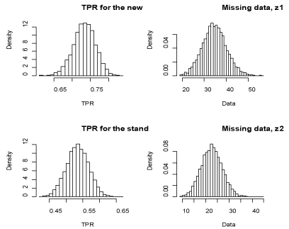
Figure 1 Posterior distributions of the TPRs and the missing data under conditional independence of the tests.
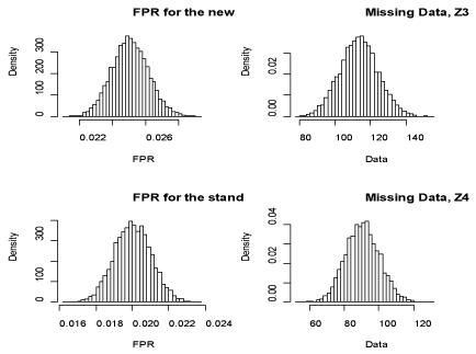
Figure 2 Posterior distributions of the FPRs and the missing data under conditional independence of the tests.
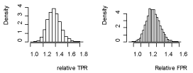
Figure 3 Posterior distributions of the relative TPR and relative FPR of the tests under conditional independence of the tests.
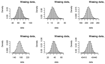
Figure 4 Distributions of the missing data.

Figure 5 Distributions of the relative TPR and relative FPR of the tests under dependence of the test.

Disease Status


D = 1

D = 0


Test 2

Test 2


X2 = 1

X2 = 0

Total

X2 = 1

X2 = 0

Total

Randomized to receive test 1 first

Test 1


X1 = 1

n1111

n1101

n11.1

n1011

n1001

n1001

X1 = 0

z0111

z0101

z011

z0011

z0001

z001

Total

?

?

?

?

?

?

Randomized to receive test 2 first


Test 1


X1 = 1

n1112

z1102

?

n1012

z1002

?

X1 = 0

n0112

z0102

?

n0012

z0002

?

Total

n.112

z102

?

n.012

z102

?

Table 1 Data from a Randomized Paired Screen Positive Design


D=1

D=0

Test Outcome, Y

Test Outcome, Y

Positive

Negative

Total

Positive

Negative

Total


Test

Test X1

n111

n110

n11.

n101

n100

n10.

Test X2

n011

n010

n01

n001

n000

n00

Total

?

?

n1

?

?

n0

Table 2 Summarized data from RPSP design when the tests were assumed to be conditionally independent


Diseased, D=1

Non-Diseased, D=0

Test X2

Test X2

Positive

Negative

Total

Positive

Negative

Total


Test X1

Positive

n111

n110

?

n101

n100

?

Negative

n011

n010

?

n001

n000

?

Total

?

?

?

?

?

?

Table 3 Summarized data from the RPSP design when the tests were assumed to be dependent

95% Credible bounds
Estimator Estimate variance Lower Limit Upper Limit
TPRX1 0.73 0.0009 0.67 0.79
TPRX2 0.53 0.0012 0.47 0.6
FPRX1 0.025 1.29E-06 0.023 0.027
FPRX2 0.02 1.01E-06 0.018 0.022
Z2 35 31.01 25 46
Z3 23 20.56 15 32
Z5 114 119.74 93 136
Z6 91 93.378 73 111
TrPRX1:X2 1.38 0.0109 1.19 1.59
FrPRX1:X2 1.25 0.0075 1.09 1.43

Table 4 Estimates of the measures of accuracy for the two screening test under the assumption of conditional independence

The point estimates and the 95% credible bounds of the parameters of the Dirichlet posterior distribution, the measures of accuracy and the missing data were also computed and the results were as shown in (Table 5). The relative TPR was computed as ((pi1+pi2)/(pi1+pi3)) while the relative FPR was computed as ((pi4+pi5)/(pi4+pi6)) which are the probabilities of the appropriate cells in (Table 3).

Discussions, conclusion and recommendations

When the tests were conditionally independent the TPR of the new screening test was estimated to be 0.73 while that of the standard test was estimated to be 0.53. Thus the relative TPR of the new screening test to that of the standard test was 1.38(95% credible bounds: 1.19, 1.59). When the missing data was ignored the disease detection probability (DP) of the new screening test was 0.58 while the DP of the standard screening test was 0.44. This gives a relative TPR of 1.34(95% credible bounds: 1.12, 1.62). The relative TPR obtained when the missing data was ignored was different from that obtained when the missing data was ignored indicating downward bias.

The FPR of the standard screening test was estimated to be 0.02 while that of new screening test was estimated to be 0.025. Thus the relative FPR of the new screening test to that of the standard screening test was 1.25(95% credible bounds: 1.09, 1.43). The false referral probability (FP) of the new screening test when the missing data was ignored was 0.016 while that of the standard screening test was 0.02 giving a relative FPR of 1.25(95% credible bounds: 1.09, 1.43). There seems to be small effect on the relative FPR when the missing data was ignored since the estimate accounting for missing data is similar to that ignoring the missing data. When the tests were treated to be dependent of each other the relative TPR and the relative FPR of the new to the standard screening tests were 1.50(95% credible bounds: 1.35, 1.67) and 1.2595% credible bounds: 1.15, 1.36 respectively. The relative TPR and the relative FPR when the missing data were ignored were 1.37(95% credible bounds: 1.27, 1.47) and 1.25(95% credible bounds: 1.14, 1.36) respectively. Apparently when the missing data were ignored, the relative TPR was downward biased while the relative FPR was not biased. Estimation ignoring the missing data leads to the estimation of the DP and FP because the number of subjects who (would have) screened negative due to one screening test and positive due to the other is not taken into account to estimate the TPRs. This means that the estimates obtained are biased. Since the assumption was that the TPR of the new screening test is 0.75 and that of the standard screening test is 0.5 the relative TPR is 1.50 which is higher than that obtained when the tests were considered to be conditionally independent from each other. This value is, however, similar to that obtained when the tests were considered to be dependent of each other which were precisely found to be 1.496. Similarly, the FPR of the standard screening test was assumed to be 0.02 and that of new screening test was estimated to be 0.025. Thus the relative FPR of the new screening test to the standard screening test was 1.25. We find that the relative FPRs in all the settings (the assumed values, under conditional independence and under dependence of the tests) are similar.

95% Credible Bounds

Estimator

Point Estimate

Variance

Lower bound

Upper Bound

Pi1

0.00379

8.32E-08

0.00325

0.00436

Pi2

0.00377

8.46E-08

0.00322

0.00435

Pi3

0.00126

2.76E-08

0.00097

0.00161

Pi4

0.00052

1.18E-08

0.00034

0.00076

Pi5

0.02428

5.07E-07

0.0229

0.02572

Pi6

0.01931

4.08E-07

0.01805

0.02056

Pi7

0.00091

1.93E-08

0.00066

0.00121

Pi8

0.94616

1.15E-06

0.94407

0.94819

Z2

69

70.47

53

86

Z3

14

33.47

7

22

Z5

227

217.24

197

257

Z6

182

183.21

156

209

Z7

42

40.64

31

56

Z8

43435

40.64

43421

43446

1.5

0.0065

1.35

1.67

1.25

0.0029

1.15

1.36

Table 5 Estimates of measures of accuracy and the missing data for the two screening tests

In this study the missing data have been simulated. This means that the TPRs and the FPRs are estimable under the assumptions stated. Therefore, we can no longer estimate the DP and the FP as demonstrated in this study. This is an achievement from this study. As to whether the observed differences in the estimates of relative TPR are true or just due to chance a statistical assessment needs to be conducted. It is recommended that if the tests are known a priori to be dependent or conditionally independent of each other it is good practice to estimate the measures of accuracy in that setting. This is because there is clear evidence from the study that the estimates are affected by the association of the tests. The relative TPR and the relative FPR resulting after the missing data were included in (Tables 2 & 3) can be interpreted as the ratio of two posterior averages. Although these are the “best” posterior estimates of the measures of accuracy, the ratio of these posterior estimators are not necessarily the best posterior estimates. Thus, Bayesian alternatives of obtaining the relative accuracy are warranted.

Acknowledgments

None.

Conflicts of interest

Authors declare that there are no conflicts of interests.

References

  1. Alonzo TA, Pepe MS, Moskowitz CS. Sample size calculation for comparative studies of medical tests for detecting presence of disease. Stat Med. 2002;21(6):835‒852.
  2. Alonzo TA, Braun M, Moskowitz CS. Small sample estimation of relative accuracy for binary screening tests. Stat Med. 2004;23(1):21‒34.
  3. Alonzo TA, Pepe MS. Assessing accuracy of a continuous screening test in presence of verification bias. Royal Statistical Society series. 2005;54(1):173‒190.
  4. Alonzo TA, Kittelson JM. A novel design for estimating relative accuracy of screening tests when complete disease verification is not feasible. Biometrics. 2006;62(2):605‒612.
  5. Cheng H, Macaluso M. Comparison of the accuracy of two screening tests with a confirmatory procedure limited to positive results. Epidemiology. 1997;8(1):104‒106.
  6. Albert JH, Chib S. Bayesian analysis of binary and polychotomous response data. Journal of the American Statistical Association. 1993;88(422):669‒679.
  7. Leonard T. Bayesian simultaneous estimation for several multinomial distributions. Communications in Statistics in Statistics A. 1997;6(7):619‒630.
  8. Laurence J, Gyorks TW. Inferences for likelihood ratios in the absence of a gold standard. Med Decis Making. 1996;16(4): 412‒417.
  9. Walsh B. Markov Chain Monte Carlo and Gibbs sampling. Lecture Notes for EEB 581 version 26. 2004.
  10. Johnstone J, Dinardo J. Econometrics Methods (4th edn), McGraw‒Hill International Editions, Singapore, 1997;pp. 496.
  11. Keter KA, Otieno RA, Kinyanjui KJ. Sample size for a randomized paired screen positive design. JP Journal of biostatistics. 2011;6(2):97‒108.
  12. Parimal M. Theory of Probability. New central Book Agency Ltd., Kolkota, India. 2012.
Creative Commons Attribution License

©2014 Alfred, et al. This is an open access article distributed under the terms of the, which permits unrestricted use, distribution, and build upon your work non-commercially.