The emphasis of this study is on the solar aspects of the relation between the average terrestrial Northern Hemisphere ground temperature $\Delta T_E{}_{arth}$ and the total magnetic fluxes of both the equatorial and the polar fields of the sun, characterized by their proxies, viz. the maximum value per Schwabe cycle of the Group Sunspot Number ( $G{n}_{max}$ ) and the minimum value of the global antipodal magnetic amplitude activity index aa (aamin) . The former is known for the period 1610 (beginning of systematic sunspot observations) till present and the latter from 1844 (first aa determinations) till present. In order to eliminate the effects of short–term, mainly non–solar variations such as volcanos, el Niño, while also not putting too much emphasis on the Schwabe cycle, the variables are smoothed over 18 years.

The increasingly strong ‘global warming’ (commonly called the modern temperature increase) is statistically significant after around 1915. We estimate that the variations of the terrestrial temperature between 1844 and 1910 are 43% due to those in the solar equatorial magnetic fields and 32 % due to those in the polar fields, while the remaining 25% has another (non–solar?) origin. We expect that the period of solar activity that has recently started will be of the Regular type during the present millennium.

Keywords: global warming, terrestrial temperature, magnetic fields, polar fields, solar activity, millennium, magnetic flux, equatorial field

In the first years of this century the International World Data Center (WDCJ–SILSO) proposed to improve the current Zürich sunspot numbering system, introduced by Wolf, developed further by Waldmeier and successors: the Wolf Sunspot Numbers, generally called International Sunspot Number; ISN. It was proposed to replace it by a new system of sunspot counting (the Modified International Sunspot Numbers (MISN).^1,2 Around the same time another proposed counting system was introduced; it is called the Group Sunspot Numbers (GSN).^3–5

The main reason for the change to the modified international sunspot numbers was to overcome the ‘Waldmeier discontinuity’,⁶ while the introduction of the Group Sunspot Numbers was based on the fairly generally accepted point of view that sunspot groups represent solar equatorial magnetic variability better than the Zürich system, the latter being based on a combination of counts of individual spots and groups of them. In this paper we distinguish between the three systems by the above names with acronyms: ISN, MISN and GSN and the corresponding mathematical symbols^1,2 Ri, Sn, and Gn. We will chiefly make use of the maximum values per Schwabe cycle (Table 1) of the last of these variables: $G{n}_{max}$ . This variable will be used as the proxy for the total equatorial magnetic flux.

The suggested modifications demand to be checked in various ways. In a previous paper⁷ we compared the average terrestrial northern hemisphere ground temperatures $\Delta T_{Earth}$ with $R{i}_{max}$ and$a{a}_{min}$ , but here we present a redetermination of the dependence of the observed average terrestrial Northern Hemisphere Earth’s ground temperature on proxies for both the equatorial and the polar solar magnetic field as follows:

For the equatorial field we selected$G{n}_{max}$ . We choose it instead of $S{n}_{max}$ , not only because the group numbers are expected to be a better proxy for the equatorial magnetic field than the MISN, but also because the listings of the International Data Centre only give the MISN for the period 1700 to present, while the GSN are available since 1610. A longer period of measurements is an argument for expecting a better accuracy. Also, it is precisely during the major part of the 17^th century that solar activity went through a deep minimum, the Maunder Minimum. Thus, since the range of GSN values is considerably broader than that of the MISN, we might also expect a better accuracy of the mathematical results. 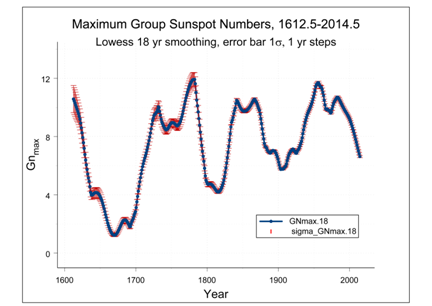Hence, we choose $G{n}_{max}$ as our proxy for the equatorial component. These are smoothed by a running 18 years smoothing time interval; cf. Figure 1 (the choice of these 18 years will be explained in Section 2 of this paper; ref. Figure 3).

Following Russell et al.⁸, Russell & Mulligan⁹, Mayaud et al.¹⁰ we introduced $a{a}_{min}$ as a proxy for the polar magnetic field strength fluxes in this study, while realizing that most researchers of this theme restrict themselves to the equatorial field. But earlier, we have stressed that the total polar magnetic fluxes, being roughly of the same order of magnitude as the total equatorial fluxes, should be included in the investigation.^11–13

Figure 1 Annual average values of the maximum Group Sunspot Numbers$G{n}_{max}$ , smoothed by the Lowess technique (Cleveland et al.29 as described in Section 2) with a running 18 years smoothing time interval. The sigma values are based on the observed standard deviation values for the individual data; they are modified by the interpolation between the maxima and by the Lowess filtering (as described in the last paragraph of Section 2).

We justify this assumption later in this paper. The various aspects of polar activity, such as the polar faculae, polar bright spots with their ephemeral surrounding regions and parts of the areas covered by coronal holes¹⁴ are too important for the sun–climate relationship to be neglected a priori. These proxies of the polar field strength fluxes $a{a}_{min}$ are not affected by the new system of sunspot numbering and hence they remain unchanged as compared to previous research. Reliable data for aa are only known after 1844,^8–10 while Nevalinna et al.¹⁵ proposed an extrapolation down to 1610. The combined results for the period 1610.5 to 2007.5, are shown in Figure 2, in which a 1957 discontinuity has also been taken into account.^16,17

Figure 2 Annual$a{a}_{min}$ data used in this investigation and smoothed in the same way as was done with$G{n}_{max}$ . The$a{a}_{min}$ data are only reliable after 1844; their extrapolated values from 1844 down till 1610 show a relatively large increase of sigma. We will not use these extrapolated data in our regressions.

The present study and the previous one have a precursor: De Jager et al.¹⁸ studied the relation between $\Delta T_{Earth}$ and solar equatorial (with proxy$R{i}_{\max }$ ) and polar magnetic activity and the average northern hemisphere terrestrial ground temperatureT_E. It is written as:

$\Delta T_{Earth}=x\cdot R{i}_{\max }+y\cdot a{a}_{\min }+z\cdot time+const$ ,(1)

Where all variables are smoothed over the running 18 years smoothing interval. In a later study⁷ the z·time term was initially neglected, but it has been determined thereafter from the residue. We also follow this approach in the present investigation and we will return to this topic in Section 5. In our 2010 paper each of these seven data sets was investigated by two independent methods. Hence that study yielded 14 independent values for x and y, each with their own standard deviations. It was satisfactory to see that the standard deviation of the average of these fourteen determinations was about the same as the average of the fourteen standard deviations, both for those of x and y. In conventional error theory such an agreement between the ‘internal’ and the ‘external’ mean errors is generally considered as supporting the reliability of the investigation.

The data from the above study have been used by De Jager et al.⁷ for a continuation of the investigation. That study was still based on the (unmodified) International Sunspot Numbers (ISN). Instead of using 7 separate files, we used the weighted averages of the results as given in De Jager JH et al.¹⁸ The temperature file that we use here consists of the Northern Hemisphere ground temperature data from Moberg et al.¹⁹ extended with data.^20–24 Henceforth, for shortness, we will call this data set the Moberg–Brohan file, with the symbol$\Delta T_{Earth}$ .

Our approach differs from others such as that of Jungclaus et al.²⁵ who ascribed the short–term pre–industrial temperature variation to the carbon cycle and who introduced volcanic eruptions and other short–term events to explain the occasionally observed cooling trends such as the Maunder Minimum. Certainly, these effects do occur. We have used a low–pass filter of 18 years to avoid the inclusion of relative short time effects while still including relatively long–term variation in terrestrial temperatures.

In this paper we deal with the last two and four centuries, but since Sanchez–Sesma et al.²⁶ found that solar activity, similar to the present one, existed during a multi–millennial (~9500 years) period, and Luthardt L et al.²⁷ found that the Schwabe cycle even did occur over a period as long as 290 Myrs, we expect that our results may also apply to a period, longer than these four centuries, but that assumption will not be used elsewhere in this paper.

The 18 years that we selected for the smoothing interval was initially derived by De Jager et al.²⁸ who found this to be the most efficient way of smoothing, eliminating short time effects mentioned earlier. We verified this by deriving the Northern Hemisphere variation of the average ground temperature, smoothed according to the Lowess technique²⁹ by a number of arbitrarily chosen smoothing intervals, viz. 4, 6, 9, 12, 18, 27 and 36 years. The results are shown in Figure 3.

Figure 3 The dots are the values of$\Delta T_{earth}$ for the years 1612 – 2011, showing the data file that we call the Moberg–Brohan temperature file. The seven full–drawn curves are interpolated, smoothed with different time intervals, with durations in years as labelled to the curves. Note the downward peak at 1816: ‘the year without a summer’.

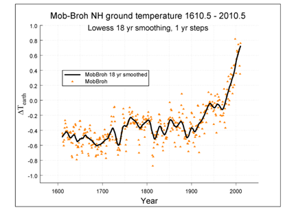
A way to examine which of these intervals is most suitable for our purpose is by looking at the smoothed temperatures around some important volcanic eruptions. To that end we primarily considered the year 1816, which is the year after the Tambora volcanic explosion, the largest eruption in historic times. In Europe the year 1816, one year after the eruption, is often called the year without a summer. Other, slightly smaller eruptions, such as 1901 Mt Pelé, 1980 Mt St Helens and 1991 Pinatubo were also considered. The study of these curves show that 4 to 12 years are too short for an acceptable smoothing interval–the dips in the curves around 1816 are still well visible, while 36 years is unnecessarily long; 18 or 27 years seem acceptable values, but longer variations in time of e.g. oceanic movements will still be observable. The diagram of Figure 4 presents the 18 years smoothed $\Delta T_{Earth}$ curve in comparison with the annual temperature data (the points). It is this temperature curve that is used in this investigation.

Figure 4 The annual$\Delta T_{earth}$ data, smoothed according to the Lowess technique by the selected 18 years running smoothing interval.

The variance of the data set is influenced by linear interpolation and by Lowess smoothing. After linear interpolation between the maxima (or minima), to obtain a year grid of$G{n}_{max}$ and $a{a}_{min}$ , the variances of neighbouring points have different values. The observed variance ${\sigma }^2{}_{y_1}$ of the line start point (x₁,y₁) and the observed variance ${\sigma }^2{}_{y_2}$ of the line end point (x₂,y₂), will determine the total interpolated variance ${\sigma }^2{}_y$ for a point (x,y) by:

${\sigma }_y^2={\left(\frac{x_2-x}{x_2-x_1}\right)}^2{\sigma }_{y_1}^2+{\left(\frac{x-x_1}{x_2-x_1}\right)}^2{\sigma }_{y_2}^2$ (2)

After interpolation Lowess smoothing has been applied. The use of Lowess smoothing reduces the variance of the measurements. The influence of the 18 year Lowess smoothing window has been calculated by the same tri–cube weight function (NIST web–based Engineering Statistics Handbook, Chapter 4.1.4.4) as was used by the Lowess smoothing of the data points.

There is consensus that the later part of the 20^th century was dominated by a fairly steep temperature increase.^30–33 This ‘modern temperature increase’ is usually ascribed to human activities. But there are different opinions regarding the time of its beginning. In our previous investigation⁷ we found that significant deviations from those data that are mainly due to solar contributions started around 1900. In contrast to that, some other authors place the beginning of the modern temperature increase at earlier times. In Jones et al.²¹ one reads about an increase that was assumed to have started mid–19^th century. Another example is found in the much cited press release of the International Astronomical Union of August 8, 2015. It states that “rising global temperatures since the industrial revolution cannot be attributed to increased solar activity”. The industrial revolution is commonly placed somewhere between the years 1760 and 1830. More citations in that sense could be made.¹⁶ For climatological investigations it is necessary to know with some precision when this additional, modern temperature increase started and how it developed. Next to solving Equation (1), the answer of the question of the starting year of the modern temperature increase is the other aim of this Section.

In our previous investigations we represented the average Northern Hemisphere ground temperature $T_{Earth}$ by the relation given by Equation (3), hence without the z·time–term. We want to use that equation again, but in this paper we will write $G{n}_{max}$ for the maximum values of the Group Sunspot Numbers.⁵ It come as a replacement of the earlier used symbol $R{i}_{max}$ . The data are interpolated and smoothed as described in Section 2. The $a{a}_{min}$ data (Figure 2) were handled the same way. Hence, the equation that we want to solve is

$\Delta T_{Earth}=a\cdot G{n}_{\max }+b\cdot a{a}_{\min }+const$ , (3)

Where the three variables ( $\Delta T_{Earth}$ ,$G{n}_{max}$ and $a{a}_{min}$ ) are presented in Figures 1, 2 & 4. With the data, thus available, Equation (3) can be solved with a least squares method of curve fitting.³⁴ In that exercise we meet two foreseeable and well–known problems, also known from our earlier investigations. First, the $G{n}_{max}$ and$a{a}_{min}$ data are fairly strongly correlated (Figures 1 & 2) and this is visible in the resulting mean errors of the parameters a and b. The other problem is that, when using the full data set from 1612 to 2007, the resulting values for a and b have fairly large mean errors, the reasons being the uncertainty of the aa data before 1844 and the increasingly large upward trend of the Earth’s average ground temperature in the course of the 20^th century, which is additional to the sun–dependent contribution. That rapid upward trend of the temperature leads to fairly large standard deviations in the resulting values of a, b and const, when using the linear equation 3 in those cases that the last year of the data set is chosen later than the beginning of the 20^th century. This is shown in the following example.

We do the calculations as described by Equation 3 for the input data sets shown in Figure 1, 2 & 4, first for data covering the full period 1844–2007, and thereafter for those covering periods between 1844 and an ‘ending year’ chosen earlier than 2007. We followed the above described approach for 12, more or less arbitrarily chosen ending years of the analysis, selected between 1882 and 2007. For each of them Equation 3 was solved for a, b and const, which thus yielded values for the relevant constants (Table 2). Equation 3 can be solved by writing it in the normal error regression matrix model Equation (4).

$Y=X\beta +\epsilon$ , (4)

The variables in this model are:

$Y=\left[\begin{array}{c}\Delta {\text{T}}_{{\text{Earth}}_{\text{1}}}\\ \Delta {\text{T}}_{{\text{Earth}}_{\text{2}}}\\ ⋮\\ \Delta {\text{T}}_{{\text{Earth}}_{\text{n}}}\end{array}\right]$ ,$X=\left[\begin{array}{ccc}G{n}_{{\max }_1}& a{a}_{{\max }_1}& 1\\ G{n}_{{\max }_2}& a{a}_{{\max }_2}& 1\\ ⋮& ⋮& ⋮\\ G{n}_{{\max }_n}& a{a}_{{\max }_n}& 1\end{array}\right]$ ,$\beta =\left[\begin{array}{c}a\\ b\\ const\end{array}\right]$ ,$\epsilon =\left[\begin{array}{c}{\epsilon }_1\\ {\epsilon }_2\\ ⋮\\ {\epsilon }_n\end{array}\right]$

Matrix X is the design matrix, vector$\epsilon$ is a vector of independent random variables with the mean value$E\left\{\epsilon \right\}=0$ and variance${\sigma }^2\left\{\epsilon \right\}={\sigma }^{2}I$ , and is the identity matrix. The solution of the regression model in Equation (4) can be written as:

$\widehat{Y}=X\beta$ , with $\beta =\left[\begin{array}{c}a\\ b\\ const\end{array}\right]={\left(X^{\prime }X\right)}^{-1}{X}^{\prime }Y=AY$ (5)

Here $\widehat{Y}$ is the fitted value and$A$ is the well–known Moore–Penrose pseudo inverse. The residual terms$\epsilon$ can be calculated as:

$\epsilon =Y-\widehat{Y}=Y-XAY=\left(I-XA\right)Y$ (6)

The residual standard deviation of the fit model${\sigma }_{\text{model}}$ is the, in our case for Lowess smoothing corrected, standard deviation of vector$\epsilon$ , is defined as the positive root out of the corrected “error mean square” (MSE):

${\sigma }_{\text{model}}=\sqrt{MSE}=\sqrt{\frac{SSE}{df}}=\sqrt{\frac{{\displaystyle \sum _{i=1}^n{\left(y_i-{\widehat{y}}_i\right)}^2}}{n-p-\lambda }}$ ,(7)

Where the SSE is the “error sum of squares” or “residual sum of squares”. The part n–p, indicates the degrees of freedom, which is the number of measurements minus the number of regression parameters. We add that the 18 years Lowess smoothing (as is done in this investigation) results in diminishing of the number of ‘independent‘ observations, so that the term n–p leads to a smaller number of degrees of freedom. The added number of equivalent regression parameters $\lambda$ , which extra decrease the number of the degrees of freedom, are calculated with Cleveland’s approximation, by

$\lambda =2+\frac{2}{f}$ (8)

Here $f$ is the relative filter span with respect to the number of measurements. For example an 18 year window and a measuring period of 164 years with one year per point, gives $f=18/164=0.110$ . For this $f$ value we compute $\lambda =20.22$ .

With the above data the total of the residual sum of squares of the differences between observed and model temperatures (SSE) was derived. These data are not directly mutually comparable because the degrees of freedom of the various sets of data are different for the various ending years. But the positive root of their quotient SSE/df , here called ${\sigma }_{model}$ (third column of Table 2), is a comparable quantity.

$df=n-\lambda -p$ (9)

The decomposed standard deviations ${\sigma }_a$ ,${\sigma }_b$ ${\sigma }_{const}$ and of the regression model can be determined by calculating the variance–covariance matrix of the regression coefficients.³⁴ The result of the estimated value of this matrix is:

$s^2\left\{\beta \right\}=A{\sigma }^2\left\{Y\right\}{A}^{\prime }=MSE\cdot {\left(X^{\prime }X\right)}^{-1}$ (10)

The values of the decomposed variances are on the main diagonal of the $s^2$ matrix. Columns 4 till 6 of table I show the square roots of these values. Note that the MSE is the for Lowess smoothing corrected MSE, given in Equation (7).

The adjusted values of the coefficient of determination $R_{adj}^2$ (last column of Table 2) indicates the fraction of the variance that is explained by the model. It is solved with:

$R_{adj}^2=1-\frac{SSE}{SSTO}\frac{n-1}{n-\lambda -p}$ (11)

Here SSE = residual – or error sum of squares, SSTO = total sum of squares (SSE + SSR, with SSR = the sum of squares of the regression around the mean), n = total number of measurements involved in the regression. Here n=164 and p is the number of degrees of freedom involved in solving the equation; here p = 3,$\lambda$ and is the equivalent number of parameters used by the Lowess technique, (cf. Equation (8)); here $\lambda =20.22$ .

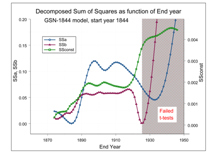
A straightforward conclusion from Table 2 is that the non–solar upward trend in the temperature (the ‘modern temperature increase’) had a starting date around 1910–1920. This result finds support in a study from Love et al.^35,36 who also find that during the main part of the 20^th century “an anthropogenic signal is hiding correlation between solar–terrestrial variables and global temperature”. This result is also understandable when realizing that their study was restricted to the fairly short period from 1860 to present. The resulting standard deviation values (third column of Table 2) show that the smallest relative residual squared differences are found for ending years before 1924. This effect can also be shown in a graph, Figure 5, where the decomposed sums of squares are a function of the ending year.

Figure 5 The decomposed sum of squares as a function of the ending year. The grey zone is the region where several t–tests failed (see chapter 4 for more information), because of the disturbing influence of the modern temperature increase at the solar model regression. The blue SSa curve belongs to the sum of squares (SS) of$G{n}_{max}$ , the red SSb curve to the SS of$a{a}_{min}$ , and the green SSconst curve to the SS of the constant and is also called SSE.

The green SSconst curve in Figure 5 is the sum of squares with regard to the constant or the earlier defined SSE in Equation (7), which is proportional with the variance of the residual sum of squares. It is clearly visible that the value drops to a lower and more constant value before 1920. Also the sum of squares of the other proxies, show the same behaviour. The main conclusion is that the modern temperature increase started somewhere around 1920.

Figure 5 shows also a drop of all sums to about zero before 1890, but with a bad t–test for ‘constant’ a, as can be seen in the last row of Table 2. This means that regression with both proxies fails in this region with the GSN–1844 model data. It can be a hint that the physical mechanism that regulate the sun induced temperature variation uses high order terms of the proxies. It is a topic for further study.

Now we choose from Table 2, with the aid of adjusted coefficient of determination, the end year of 1910 for the model; we call this model the GSN–1844 model, with the following parameters (cf. Table 2):

$a=0.1160\pm 0.0177$

$b=–0.0620\pm 0.0118$

$c=–0.6761\pm 0.0348$

Hence, Equation (3) should also be solved for input data covering an earlier period, for which we took 1612–1910. Now the model has to be changed by assigning b=0, because of the unreliable $a{a}_{min}$ data before 1844. For these input data we found (cf. Table 3):

$a=0.0205\pm 0.0017$

$c=–0.5615\pm 0.0124$

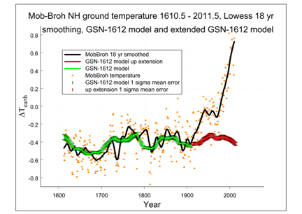
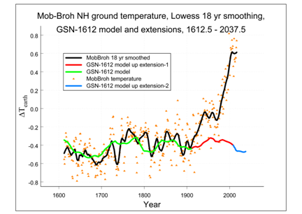
We will refer to this model as the GSN–1612 model that we use in the later part of this paper. On basis of the GSN–1612 model Figure 6 was drawn. It gives the relation between the temperature variations due to solar activity (the green GSN–1612 curve with the red extension beyond 1910) as compared with average Northern Hemisphere ground temperature (the black MobBroh 18 yr smoothed curve). The modelled sun–induced part is based on Equation (3) and the GSN–1612 model for data restricted to the period before 1910. The modern temperature increase is well visible in Figure 6 and ranges up to nearly one degree centigrade at the beginning of the 21^th century.

Figure 6 Variation of the smoothed average Northern Hemisphere ground temperatures (black MobBroh 18 yr smoothed curve) as compared with sun–induced values (green GSN1612 model curve with red extension after 1910).

As explained earlier in this paper, these numbers have been corrected for the reduction in degrees of freedom due to the Lowess averaging process. The total variance of the model and the proxies can be found with the error propagation formula and is:

${\sigma }_{\Delta T_{earth}}^2=G{n}_{\max }^2{\sigma }_a^2+a^2{\sigma }_{G{n}_{\max }}^2+a{a}_{\min }^2{\sigma }_b^2+b^2{\sigma }_{a{a}_{\min }}^2+{\sigma }_{const}^2$ (12)

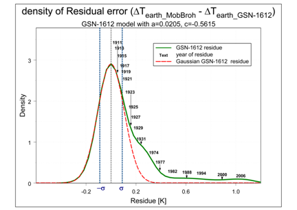
The total error is visible in Figure 6 as the thin coloured bands around the solar model curves. We next consider the residuals corresponding to the data derived for Equation (3) and the GSN–1612 model. They have the character of a function giving the change density as presented in Figure 7. This diagram shows that the residuals explosively exceed the one–sigma limit after the year 1915. This confirms the conclusion as found in the third column of Table 2.

Figure 7 Residuals of the numerical representation of the terrestrial temperature data by Equation (2), as presented in Figure 6. The essential part of the curve is its tail; there the years given are those of the residues. In the normal region the curve gives the addition of residues of more years, as is usually the case. The curve shows the deviation from the normal distribution.

As appears from Figure 6 the long–term variations in the average Northern Hemisphere terrestrial ground temperature before ~1915 are well correlated with the long–term variation of solar activity. It is shown by Figure 6 that the additional modern temperature increase has presently already reached a value of 0.9 K above the expected value for solar influence (Figures 6 & 7). The physical explanation of this observation is a problem for climatology, that has already been studied by many climatologists and that therefore will not be discussed again at this place.

As appears from Figures 1 & 2 the two proxies are fairly strongly correlated and this leads to the question of the reliability of the results described in the preceding Sections. We examine this by deriving the regressions between various combinations of Equation (3) as shown in Table 3. The first one refers to the long data set model GSN–1612 with only proxy$G{n}_{max}$ , the subsequent three of them refer to data for the period 1844–2007, and the next three to those for the period 1844–1910 with the GSN–1844 model. For the first period we derived the regression for one proxy; for both other periods we derived the regressions for three cases: the two proxies, then for$G{n}_{max}$ only and finally for $a{a}_{min}$ only. All these input data have been smoothed, as described earlier in this paper, by the 18 years Lowes’s procedure.

The results are given in Table 3. It gives for the 7 cases the fitted coefficients, the t–value, the value of the adjusted coefficient of determination$R_{adj}^2$ , and the correlation between the coefficients of the proxies for the various cases. The t–value is the ratio between the mean value of the coefficient and the standard error of the coefficient; the value t~2.6 indicates 99% confidence. In other words the study of these data for the interval 1844 – 2007 with the two proxies shows that the t–value is too low ($t<2.6$ ) with a 1.0 % probability that the coefficient of proxy $G{n}_{max}$ is not different from zero. When single proxies are used, the adjusted coefficient of determination $R_{adj}^2$ with the proxy $a{a}_{min}$ shows 13.9% better explanation of variance by the model and is therefore the more acceptable one.

For the shorter time interval (1844–1910) the two proxies used together would fit best. The use of only the $G{n}_{max}$ proxy gives, according to the $R_{adj}^2$ fraction, 29.4% explanation. The addition of the $a{a}_{min}$ proxy gives 52.2 % explanation or 22.8% additional support for the solar influence on the terrestrial ground temperature$\Delta T_{earth}$ .

Table 3 shows therefore that the influence of the correlated proxies can be separated; in any case that such is the case for the shorter time interval.

As a next step we also want to examine the relative roles to global warming by the equatorial and polar magnetic fields. When doing that we must take into account (Figures 6 & 7) that considerable part of the data after 1910 is not due to solar effects; actually these are only valid for the data from 1844 till 1910, while the solar origin of the data from before 1844 is questionable. For this exercise we have to calculate the partial adjusted coefficient of determination, which gives the conditional proportion of variation explained by proxy$G{n}_{max}$ that cannot be explained by proxy $a{a}_{min}$ , as:

$R_{adj\_G{n}_{\max }|a{a}_{\min }}^2=1-\frac{SSE\left(G{n}_{\max },a{a}_{\min }\right)}{SSE\left(a{a}_{\min }\right)}\frac{n-\lambda -p_{a{a}_{\min }}}{n-\lambda -p_{G{n}_{\max },a{a}_{\min }}}$ (13)

The other way round, the variation explained by proxy $a{a}_{min}$ cannot be explained by $G{n}_{max}$ :

$R_{adj\_a{a}_{\min }|G{n}_{\max }}^2=1-\frac{SSE\left(G{n}_{\max },a{a}_{\min }\right)}{SSE\left(G{n}_{\max }\right)}\frac{n-\lambda -p_{G{n}_{\max }}}{n-\lambda -p_{G{n}_{\max },a{a}_{\min }}}$ (14)

Here$SSE(G{n}_{max},a{a}_{min})$ = the residual SS in a regression with $G{n}_{max}$ and$a{a}_{min}$ , $SSE(a{a}_{min})$ = the residual SS in a regression with only proxy$a{a}_{min}$ , $SSE(G{n}_{max})$ = the residual SS in a regression with only proxy$G{n}_{max}$ , and again n = total number of measurements involved in the regression; here n=67,$p_{a{a}_{min}}$ , $p_{G{n}_{max}}$ and $p_{G{n}_{max},a{a}_{min}}$ = the number of degrees of freedom involved in solving the equation; here $p_{a{a}_{min}}=2$ ,$p_{G{n}_{max}}=2$ and$p_{G{n}_{max},a{a}_{min}}=3$ , and $\lambda =9.44$ is the equivalent number of parameters used by the Lowess technique, (Equation (7)).

We have calculated from the last 3 regressions with GSN–1844 model in Table II, the$SSE\left(G{n}_{max},a{a}_{min}\right)$ with 2 proxies and both the$SSE\left(G{n}_{max}\right)$ and$SSE\left(a{a}_{min}\right)$ with one proxy. With Equations (13 & 14), while using the calculated SS data, the partial adjusted coefficients of determination are calculated. Table 4 shows the SSE data and the results of the partial adjusted coefficient of determination. In the time interval 1844 till 1910, the proxy$G{n}_{max}$ explains 42.9% of the variance, that$a{a}_{min}$ doesn’t explain, and the proxy $a{a}_{min}$ explains 32.4% of the variance, that $G{n}_{max}$ doesn’t explain.

This leads to the conclusion that during 1844 to 1910 the terrestrial temperature variation was for 42.9% related to variations in the equatorial magnetic fields and for 32.4% to those on the polar fields while the remaining 24.7% has other causes. This latter aspect should certainly invite further research. That is a theme for climatological research and will not be discussed here.

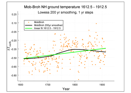
We now make a 200 year Lowess smoothing of the input ground temperature data of $\Delta T_{Earth}$ in order to examine how the long–term temperature changed in the period 1612 to 1912, i.e. without the modern temperature increase described in previous Sections. We then apply a linear fit to the resulting curve of the smoothed temperature data, such in order to determine the slope.

Figure 8(A) shows a black smoothed MobBroh temperature curve and a green linear fit. A positive slope is visible in the 200 years smoothed Mob–Broh ground temperature data$\Delta T_{Earth}$ between the years 1612 and 1912. The linear fit of the smoothed data has a slope $0.0582\left(\pm 0.0019\right)K$ of per century.

Figure 8(A) The linear rest term suggests a Hallstatt–type contribution. The sine–like signal indicates a Suess–type contribution.

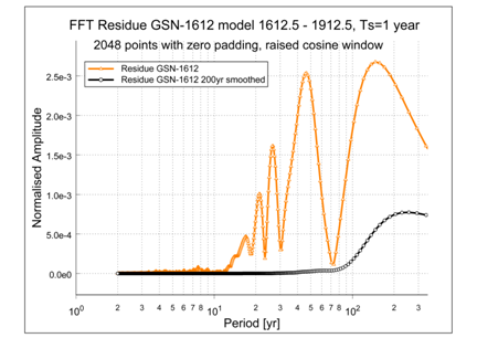
There is also a cyclic signal visible, which that oscillates around the linear fit. The period of the latter appears to be only slightly longer than the 210 years Suess /de Vries cycle. We now make an FFT of the signals in Figure 8A, shown in Figure 8B, to confirm this period.

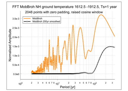
Figure 8(B) The FFT of the signals shown in Figure 8A. The MobBroh data set contains more signals than the quasi–periodicities of the solar cycle in Table 1. It is clearly visible that the Lowess filtering weakens the signals with a period shorter period than 200 years.

The resolution of the FFT is enhanced by zero padding from 301 to 2048 points, and by the use of a raised cosine window over the data. Further both data sets have been corrected with the linear fit, to prevent distortion from longer periods outside the measurement window of 300 years. It appears from the smoothed MobBroh spectrum, that the sine–like signal in Figure 8A consists of an addition of more periods. The peak period of the smoothed MobBroh signal in Figure 8B, is slightly longer than the 210 years Suess /de Vries cycle.

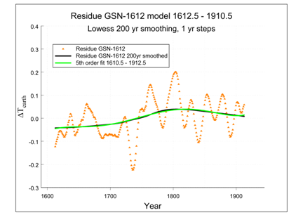
Subsequently we repeat the same steps on the 18 years residue of the GSN–1612 model, which results in Figures 9A & 9B. Again, the black curve shows the 200 year smoothed residue and the linear fit is given in green. The slope value of the linear fit is $0.0284\left(\pm 0.0010\right)K$ per century. Also, Figure 9A shows a cyclic signal, slightly longer than the Suess/De Vries cycle.

Figure 9(A) A linear fit on the residue of the GSN–1612 model suggests a Hallstatt–type contribution. Note the change in the temperature scale with respect to Figure 8A.

Now we compare Figure 8 & 9, to see in what respect the model has changed the temperature residue. The slope of the linear fit in Figure 9A is about 50% of the slope in Figure 8A (or the maximum of the smoothed amplitudes in Figure 9B is about 50% of the maximum of the smoothed amplitudes in Figure 8B); this means that the model resolves 50% of the slope. In De Jager et al.⁷ indications were also found for a slow but steady increase of the residual temperature over the centuries. A value of $0.022\left(\pm 0.001\right)K$ per century was found and that value is approximately confirmed in this study.

Figure 9(B) FFT of the residue and the Lowess filtered residue in Figure 9(A); the residue signal appears to be an addition of about five separate signals. Also the 18 years Lowess filtering is clearly visible in the residue.

Next we compare the 200 year smoothed curves in Figures 8A & 9A. The signal in Figure 9A has almost the same shape as the corresponding one in Figure 8A, but with 30% smaller amplitude. This cyclic signal, possibly the filtered Suess cycle as can be seen in the FFTs, is not completely resolved by the GSN–1612 model, because it is still partly visible in the residue after this second process. However, in the original data of the proxy $G{n}_{max}$ the Suess cycle is present and it seems that both proxies interfere with each other. Higher even order components of the proxies may solve this problem.

We now start a secondary approach by extending the GSN–1612 residue fit with higher order terms of the time variable. It appears that almost the complete residue can be resolved with a fifth order time polynomial and adjusted coefficient of determination$R_{adj}^2$ of 0.994.

The resulting curve is shown in Figure 10; the polynomial is:

Figure 10 A fifth order fit on the 200 years smoothed residue of the GSN1612 model shows a nearly perfect modelling of the residue, indicating the presence of a cycle that is likely to be identified to be a Suess cycle.

$\Delta T_{res}=c_0+c_{1}t+c_2{t}^{\text{2}}+c_3{t}^3+c_4{t}^4+c_5{t}^5$ ,(15)

with

The second order gradient is $–0.1725(\pm 0.0105)K$ per squared century and is probably in this residue related to the residual Suess cycle. We suggest a possible explanation for this small linear increase. From among the five fundamental periodicities in solar activity, viz. the Schwabe (~11 yrs), Hale (~22 yrs), Gleissberg (~80 yrs) , Suess (210 yrs) and Hallstatt cycles it is the latter, with its period of ~2300 years, that fits in the linear increase presented by Equation (3). The present Hallstatt cycle went through its mean value with a positive slope in the second half of the 20^th century. The next maximum will be reached around the year 2500. The GSN–1612 model and slope data with Equation (3) may well fit into this picture.

The conclusion of this Section is that there are some weak indications for a small steady increase of the temperature over the four centuries considered here. It amounts to$0.0284\left(\pm 0.0010\right)\times tK$ , where t is the time, expressed in centuries after 1612.5. The shape of the relevant curve suggests similarity to the Hallstatt periodicity. This suggestion emphasises the need for a thorough study of the physics of the mechanism(s) behind that solar periodicity. How does it manifest itself in solar variability and what (are) the mechanism(s)?

The physical explanation of this periodicity may be found in the suggested pulsations of the solar tachocline, which affects the solar equatorial magnetic activity,¹³ with a relatively small amplitude and with the Hallstatt period. If this interpretation of the solar driving model is indeed correct, then this physical explanation may find support in a study by Scafetta et al.³⁷ who ascribe the Hallstatt oscillation to the combined attraction by the major planets. We suggest that this attractive force influences the distance between the tachocline and the solar surface. This process is then an action that may be seen as a form of pulsation.

The extended transition that lasted from ~2005 till ~2010 is related to the start of another Grand Episode of solar activity.¹³ That recent phase transition, hence, marks the end of the 20^th century’s Grand Maximum.

The question of what episode comes next has been dealt with in various papers.^11,12,38 It was found that a Grand Minimum, such as the Maunder one, will occur only during the negative phase of the 2300 years lasting Hallstatt oscillation,^38,39 while a longer lasting Regular Episode does occur when this oscillation is positive.³⁸ Specifically, from investigating a sunspot maxima time series that lasted for nearly two millennia, it was found that the Hallstatt oscillation passed from positive to negative through its zero line around the year 900. That passing was accompanied by a change in the nature of Solar Dynamo Episodes from a long lasting Regular episode to another one. In wondering what kind that new episode will be we refer to the three millennia lasting time series of solar activity shown in Figure 2.⁴⁰ The regular episode that ended around the year 900 started in–250 and hence it lasted for ~1150 years. This confirms that a long lasting Regular Episode appears to occur during the whole positive phase of the Hallstatt oscillation. More recently Duhau S et al.⁴¹ predicted the value and the date of occurrence of sunspot maxima #26 to #31 for the forthcoming century and found that the Episode that started with Schwabe cycle #24 is indeed of the Regular type similar to the one that occurred between 1740 and 1924. More specifically, this Schwabe cycle is a Dalton type minimum. These data support the hypothesis that an Episode of the Regular type will occur during the major part of the forthcoming millennium. The consequent values of$G{n}_{max}$ and $a{a}_{min}$ will be similar to those that occurred in the 18^th and 19^th century. Unfortunately we cannot use the uncertain $a{a}_{min}$ data before 1844.

Based on the observed values of $G{n}_{max}$ , and assuming that solar activity during the next few decades will be comparable to that observed during the Dalton Minimum, we use GSN–1612 to compute the variation with time of$\Delta T_{Earth}$ in dependence of the main solar magnetic field fluxes for the expected changes in $G{n}_{max}$ as indicated in the previous Section. Of course we do not yet know the values of $G{n}_{max}$ for the cycles after cycle #24, nor will the above suggested values of $G{n}_{max}$ for the years 2010 through 2037 be exactly the same as those for Schwabe cycles #5, #6 and #7 (~1798 till 1833). The rationale of our present approach is our expectation, explained above, that the Grand Episode that has just started may be expected to begin with a Dalton type minimum. Thus, we suggest for the time interval 2007 to 2037 $G{n}_{max}$ data will be similar to those of the past Dalton minimum.

The results are presented in Figure 11 for the GSN–1612 model. It gives–again–the observed Moberg–Brohan temperature data. But next to that we give the expected values of the solar component of$\Delta T$ , as they are here extended to 2037. We stress that, while the data after ~2007 are based on a hypothesis, the earlier ones are based on straight observations.

Figure 11 Relative values of the solar–induced component of the average terrestrial surface temperature during the period 1612 to 2037, compared with the observed data from Moberg et al.¹⁹ to which the more recent data from Brohan et al.²⁰ are pasted. The calculated GSN–1612 model data after 2007 are based on extrapolations.

The main result of this exercise is that the values for the solar component of the average terrestrial ground temperatures $\Delta T_{earth}$ are expected to be fairly small in the coming decades. The decrease to that low value started already around the year 2000.

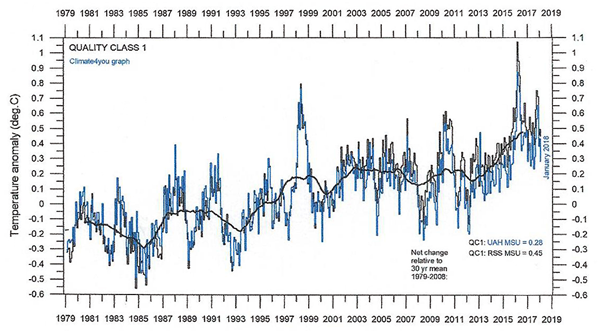
Another topic for immediate research is the question why, after the sharp rise of the average terrestrial ground temperature between ~1950 and ~2000 there came a quasi–standstill in that rise during the first decade of the 21^th century, as shown in Figure 12. We suggest that this standstill is due to the simultaneous decrease of the solar component, a decrease that started to be of some importance after ~1998, against the gradual temperature rise due to non–solar contributions, in such a way that a relative standstill in the rise of temperature occurred. What will happen after that time is a matter of speculation.

Figure 12 Global temperature variation over the past three decades, showing the remarkable standstill in the rise of temperature after ~2000 (from Ole Humlum, Temperature Report, Univ. Huntsville, 2018). This is conform Figure 11, where we also find a standstill.

This paper has two sets of conclusions. For the first we refer to Figures 6 & 7, that compares the observed average smoothed terrestrial Northern Hemisphere ground temperatures$\Delta T_{earth}$ with sun–induced values. We found that up to ~1915 the 18 years smoothed values of $\Delta T_{earth}$ are chiefly due to the sun. After 1915 a steadily increasing additional component appears which leads to increased warming. The solar component decreases in intensity in the first decade of the present century during the Transition¹³ between the 20^th century Grand Maximum and a subsequent new Episode. This explains the short relatively constant terrestrial temperature in that brief period. A near–linear increase over the four centuries studied is ascribed to the Hallstatt periodicity.

As to the future of solar activity we refer to Figure 11 and in connection with that to the exceptionally weak Schwabe cycle #24. These data in connection with the similar subsequent cycle suggest that we are presently witnessing a Dalton–type period. This may be followed by a repetition of the kind of solar activity that occurred between the years 1740 and 1924 and that we called of the Regular type. This suggests that the Grand Episode that has started with the recent Transition may also be of that type, and, as the Hallstatt oscillation changed from negative to positive in near synchronicity with the recent Solar Dynamo Transition, it would last during the rest of the current millennium as was the case during the time interval (in years) ~250 to 900 when a long lasting Regular Episode occurred⁴⁰ (Figure 2) in synchronicity with the positive phase of the Hallstatt oscillation.

We are greatly obliged to drs. Frédéric Clette and Leif Svalgaard for providing us with necessary input data. We thank Mr. F.C. Erné for his advice about the statistical approach.

The used data sets can be found at www.cdejager.com/sun–earth–publications/. Sunspot Numbers and Group Numbers data sets at: www.sidc.be/silso/datafiles.

Authors declare there is no conflict of interest.

1. Clette T, Lefevre S. Are the sunspots really vanishing? Anomalies in the solar cycle 23 and the implications for long–term models and proxies. Journal of Space Weather and Space Climate. 2012;2(A06).
2. Clette F, Svalgaard L, Vaquero JM, et al. Revisiting the sunspot number: a 400 years perspective on the solar cycle. Space Science Reviews. 2014;186(1–4):35–103.
3. Hoyt DV, Schatten KH. Group Sunspot Numbers: A New Solar Activity Reconstruction. Solar Physics. 1998;181(2):491–491.
4. Hathaway DH, Wilson RM, Reichmann EJ. Group sunspot numbers: Sunspot cycle characteristics. Solar Physics. 2002;211(1–2):357–370.
5. Svalgaard L, Schatten KH. Reconstruction of the sunspot group number: the backbone method. Solar Physics. 2016;291(9–10):2653–2684.
6. Aparicio JP, Vaquero JM, Galego MC. The proposed “Waldmeier discontinuity”: How does it affect to sunspot cycle characteristics? Journal of Space Weather and Space Climate. 2012;2(A12).
7. De Jager C, Nieuwenhuijzen H. Terrestrial ground temperature variations in relation to solar magnetic variability, including the present Schwabe cycle. Natural Sciences. 2013;5(10):1112–1120.
8. Russell CT. On the possibility of deducing interplanetary and solar parameters from geomagnetic records. Solar Physics. 1975;42(1):259–269.
9. Russell CT, Mulligan T. The 22–year variation of geomagnetic activity: Implications for the polar magnetic field of the sun. Geophysical Research Letters. 1975;22(23):3287–3288.
10. Mayaud PN. The aa–index; a 100 years series characterizing the magnetic activity. Journal of Geophysical Research. 1972;77(34):6870–6874.
11. Duhau S, De Jager C. The solar dynamo and its phase transitions during the last millennium. Solar Physics. 2008;250(1):1–15.
12. Duhau S, De Jager C. The forthcoming Grand Minimum of solar activity. Journal of Cosmology. 2010;8:1983–1999.
13. De Jager C, Akasofu SI, Duhau S, et al. A remarkable recent transition in the solar dynamo. Space Science Reviews. 2016;201(1–4):109–145.
14. Petrie GJD, Petrovay K, Schatten KH, et al. Solar polar fields and the 22–year activity cycle: observations and models. Space Science Reviews. 2014;186(1–4):325–357.
15. Nevanlinna H, Kataja F. An extension of the geomagnetic index series aa for two solar cycles (1844–1898). Geophysical Research Letters. 1993;20(23):2703–2706.
16. Lockwood M. Solar Influence on Global and Regional Climates. Surveys in Geophysics. 2012;33(3–4):503–534.
17. Lockwood M, Barnard L, Nevalinna H, et al. Reconstruction of geomagnetic activity and near–earth interplanetary conditions over the past 167 yrs–part 2: a new reconstruction of the interplanetary magnetic field. Annales Geophysicae. 2013; 31(11):1957–1977.
18. De Jager C, Duhau S, Van Geel B. Quantifying and Specifying the solar influence on terrestrial surface temperature. Journal of Atmospheric and Solar–Terrestrial Physics. 2010;72(13):926–937.
19. Moberg H, Sonechkin DM, Holmgren K, et al. Highly variable northern hemisphere temperatures, reconstructed from low–and high–resolution proxy data. Nature. 2005;433(7026):613–617.
20. Brohan P, Kennedy JJ, Harris L, et al. Uncertainty estimates in regional and global observed temperature changes; a new data set from 1850. Journal of Geophysical Research: Atmosphere. 2006;111(D12).
21. Jones PD. Mann ME. Climate over past millennia. Reviews of Geophysics. 2004;42(2):1–42.
22. Kennedy J, Good S, Tichner H, et al. Global and regional climate in 2008. Weather. 2009;64(11):288–297.
23. Kerr RA. Climate change. What happened to global warming? Scientists say just wait a bit. Science. 2009;326(5949):28–29.
24. Hansen J, Ruedy R, Sato M, et al. Global surface temperature change. Reviews of Geophysics. 2010;48(RG4004):1–29.
25. Jungclaus, JH, Lorenz SJ, Timmreck C, et al. Climate and carbon–cycle variability over the last millennium. Climate of the past. 2010;6:723–737.
26. Sanchez–Sesma J. Evidence of cosmic recurrent and lagged millennia–scale patterns and consequent forecasts: multi–scale responses of solar activity (SA) to planetary gravitational forcing (PGF). Earth System Dynamics. 2016;7:583–595.
27. Luthardt L, Rößler R. Fossil forest reveals sunspot activity in the early Permian. Geology. 2017;45(3):279–282.
28. De Jager C, Usoskin I. On possible drivers of sun–induced climate Change. Journal of Atmospheric and Solar–Terrestrial Physics. 2006;68(18):2053–2060.
29. Cleveland WS. Robust Locally Weighted Regression and Smoothing Scatterplots. Journal of the American Statiscal Association. 1979;74(368):829–836.
30. Usoskin IG, Solanki S, Schüssler M, et al. Millennium–scale sunspot number reconstruction: Evidence for an unusually active Sun since the 1940s. Physical Review Letters. 2003;91(21):211101–211104.
31. Solanki SK, Usoskin IG, Kromer B, et al. Unusualactivity of the sun during recent decades compared to previous 11,000 years. Nature. 2004;431:1084–1087.
32. De Jager C, Duhau S. Episodes of relative global warming. Journal of Atmospheric and Solar–TerrestrialPhysics. 2009;71(2):194–198.
33. De Jager C, Duhau S. The variable solar dynamo and the present solar activity; influence on terrestrial surface temperature. In: Cossia JM, editor. USA: Nova Science Publishers; 2011.  
34. Kutner MH, Nachtsheim CJ, Neter J, et al. Applied Linear Statistical Models. 5th ed. USA: McGraw–Hill Education; 2005. p. 1–1415.
35. Love TJ. Long–term biases in geomagnetic K and aa indices. Annales Geophysicae. 2011;29:1365–1375.
36. Love JJ, Mursula K. Tsai VC, et al. Are secular correlations between sunspots, geomagnetic activity, and global temperature significant?  Geophysical Research Letters. 2011;38(21):1–6.
37. Scafetta N, Milani F, Bianchini A, et al. On the astronomical origin of the Hallstatt oscillation from radiocarbon records through the Holocene. Earth–Science Reviews. 2016;162:24–43.
38. De Jager C, Duhau S. Sudden transitions and grand variations in the solar dynamo, past and present. Journal of Space Weather and Climate. 2012;2(A07):1–8.
39. Steinhilber E, Abreu JA, Beer J, et al. Interplanetary magnetic fields during the past 9399 years inferred from cosmogenic radionuclides. Journal of Geophysical Research. 2010;115(A1):1–14.
40. Usoskin IG, Hulot G, Gallet Y, et al. Evidence for distinct modes of solar activity. Astronomy and Astrophysics. 2014;562(L10):1–4.
41. Duhau S, De Jager C. On the Origin of the Dansgaard–Oeschger Events and Its Time Variability. Marine Isotope Stage 3 in Southern South America, 60 KA BP–30 KA BP. In: Gasparinim GM, Rabassa J, Deschamps V, Tonni ED, editors. Switzerland: Springer International Publishing AG; 2016. p. 23–47.
42. Duhau S, Martínez E. Solar dynamo transitions as drivers of sudden climate changes. In: Bharat RS, editor. UK: Global warming–impacts and future perspective; 2012. p. 1–20.
43. IPCC Climate Change. Working group I contribution to ARI. 2013.
44. Svalgaard L, Cliver EW, Kamide Y. Sunspot cycle 24: Smallest cycle in 100 years? Geophysical Research Letters. 2005;32(1):1–4.
45. Svensmark H, Friis–Christensen E. Variation of cosmic ray flux and global cloud coverage–a missing link in solar–climate relationships. Journal of Atmospheric and Solar–Terrestrial Physics. 1997;59(11):1225–1232.
46. Tinsley BA. The global atmospheric electric circuit and its effects on cloud microphysics. IOP Publishing Reports on Progress in Physics. 2008;71(6).
47. Draper NH, Smith H. Applied regression analysis. USA: John Wiley & Sons, Inc; 1966.