This article explores the intricate concept of time, delving into its digital and complex nature. It presents a comprehensive theoretical analysis, revealing how time's multifaceted characteristics are essential for understanding various cosmic phenomena. The study extends to the implications of these properties in the realms of Cosmic Inflation and String Theory, particularly focusing on the accelerated expansion of space. This work aims to offer a deeper perspective on the complex nature of time, enriching the existing theories in Relativity and Cosmology, and providing a novel framework for viewing time beyond traditional interpretations.

Keywords: Complex time, Imaginary time, Cosmic Inflation, Sting Theory, Space Accelerated Expansion

This paper delves into the enigmatic nature of time, a topic that has long captivated the fields of Relativity and Cosmology within physics. We propose a novel theoretical framework wherein time is treated as a complex variable, a significant departure from its traditional perception as a purely real quantity. This concept opens up a myriad of possibilities, offering a more nuanced and potent descriptive tool for cosmological models. Central to our exploration is the parameter $L_I$ , representing the length of the imaginary time dimension. We argue for its critical role in the cosmic landscape and examine its dynamic nature. While directly measuring $L_I$ may seem unfeasible, akin to a cartoon character gauging the computer rendering time of its frames, we suggest methods for its indirect estimation. By reimagining time in this innovative way, we aim to unveil new perspectives in the understanding of the universe, potentially revolutionizing established notions in string theory and the fabric of spacetime itself.

Simultaneity x present time

In everyday life, we categorize time into past, present, and future, a concept deeply ingrained in the structure of our language and perception. We view the present as our current reality, the past as a bygone existence, and the future as a yet-to-be-shaped realm. This intuitive notion, however, starkly contrasts with the principles of modern physics, as highlighted by Einstein's assertion that distinctions of past, present, and future are mere persistent illusions. This arises from the theory of relativity, which posits that simultaneity is relative—events occurring simultaneously in one frame may not in another.

A critical aspect often overlooked is the role of light's finite speed in perceiving simultaneity. In Figure 1, for instance, two observers witness two lamps (one red, one green) illuminated simultaneously by synchronized clocks. However, due to their different positions, each observer perceives a different sequence of illumination. This discrepancy underscores the influence of observation distance and light travel time.

Figure 1 Two observers that disagree about which bulb lights first.

The notion extends to astronomical observations, where events like a distant star's explosion are deemed to have occurred eons ago, regardless of Earth's observational timeline. This leads us to discern two forms of simultaneity: Relativistic, varying with speed, gravitational fields, and observational distance, and Quantum, independent of observer presence. Intriguingly, quantum entanglement introduces another dimension, where observing one of a pair of entangled particles instantaneously affects the other, hinting at a form of simultaneity transcending conventional constraints. This could, theoretically, synchronize events like the two lamps' illumination. These insights compel us to reconsider our understanding of time. While Relativistic Simultaneity aligns with the illusory nature of time, Quantum Simultaneity presents the 'Present Time' as potentially integral to deciphering the universe's workings.

Spacetime behaviour, using two dimension-space analogies

In conceptualizing spacetime, we often visualize it as digital, defined by minimum spatial (Planck length) and temporal (Planck time) units. Imagine a two-dimensional digital space: initially, it resembles a chessboard (Figure 2a), offering a simplistic, grid-like structure. However, a more dynamic representation emerges when we consider a network of interconnected circles (Figure 2b), resembling a complex web rather than rigid squares.

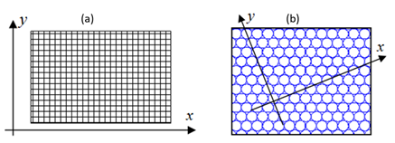
Figure 2 Two dimensions (x,y) digital space seems as:
a) A chess board; b) A network of circles.

Figure 3 extends this concept by layering these two-dimensional networks over time, akin to stacking multiple boards. This simplistic model evolves further in Figure 4, where we liken spacetime to a rectangular pool being filled with ping pong balls. Each layer of balls symbolizes a moment in time, with the topmost layer representing the present.

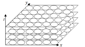
Figure 3 Two-dimension digital space being "copied" in the time.

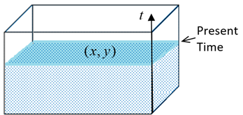
Figure 4 Analogy with a swimming pool filled by ping pong balls.

The analogy becomes more intricate in Figure 5, where varying ball sizes (representing different scales of gravitational influence) distort the straightforward layering, challenging the linear perception of time. Larger balls, akin to massive celestial bodies, create a time dilation effect, similar to that observed in Einstein's General Relativity. Here, the Planck time concept becomes variable, influenced by the gravitational field strength.

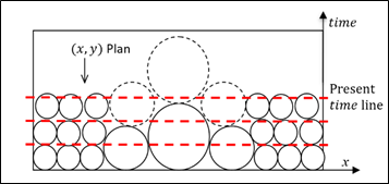
Figure 5 Analogy with a swimming pool filled by balls with different sizes.

In Figure 6, we replace balls with film reels of varying stretch lengths to illustrate time dilation visually. A fixed rate of film movement demonstrates how time progresses differently across various stretches of the film. This model correlates temporal dilation with a 'temporal velocity,' inversely proportional to the dilation factor, offering an intuitive understanding of time's fluidity in diverse gravitational fields.

Figure 6 Analogy with film reel size expansion.

Velocities in a digital spacetime

In a universe with digital spacetime, only two velocity values exist: Zero Speed $(v=0)$ and Unitary Speed $(\frac{v}{c}=1)$ , the latter being the speed of light. In a three-dimensional space $(v_x, v_y, v_z)$ , unitary speed can manifest in various forms, like negative velocity $(\frac{v_x}{c}=-1)$ or distributed across three axes $(\frac{v_m^2}{c^2}= \frac{v_x^2}{c^2}+\frac{v_x^2}{c^2}+\frac{v_x^2}{c^2}=1)$ , but the velocity's magnitude always remains unitary or zero.

This concept is vividly demonstrated in the digital universe of Minecraft (Figure 7), where the Planck distance is one meter, and the speed of light is 60m/s. In this realm, movement is quantized, a character moves in discrete steps at light speed, then remains stationary, creating an illusion of continuous motion. For instance, the skeleton in Figure 8, falling at an average speed of 6m/s actually makes intermittent jumps at light speed, punctuated by nine periods of stillness, given a mean velocity: $v_m=\frac{c}{9+1}=\frac{60}{10}=6m/s$ .

Figure 7 Space time digital universe in the Minecraft world.

Figure 8 Character living, moving and fighting in the Minecraft world.

Extending this to our universe, even a billiard ball moving at 1 m/s, essentially 'jumps' a Planck length at light speed, followed by 299792457 periods of inactivity. So, this its mean velocity will be: $v_m= \frac{c}{299792457+1}=1m/s$ . As these cycle periods are incredibly brief ($T = 299792458 \times P_t=1.61\times {10}^{-35}S$ ), our perception and instruments register it as continuous movement (Figure 8).

The only difference from Minecraft body’s movement, is that in our universe, there is no total space time velocity $(v_{st}^{})$  equal to zero, because It´s always has a unitary value $(v_s{t}^2=v_t^2+(v_x^2)/c^2+(v_x^2)/c^2+(v_x^2)/c^2=1)$ , where the time velocity $(v_{st}^{})$ can also be only 0 (body stooped in the time) or 1 (body going to future in the maximum speed) or -1 (body going to past in the maximum speed). If we consider the body’s medium velocity $(v_m)$ we obtain: $v_{st}^2=v_t^2+ \frac{v_m^2}{c^2}=1$ , meaning that in our universe one body, must chose to "jump in time" (staying still in space) or to "jump in space" (staying still in time) .

In a high-velocity scenario like a spaceship moving at 0.5c, the ship alternates between light-speed jumps and temporal stillness. Consequently, time appears dilated, exemplified by the 'film reel' analogy (Figure 9). This dilation is a direct consequence of the binary nature of digital spacetime velocities and offers an intuitive explanation for the constancy of light speed and the upper limits on material bodies' velocities.

Figure 9 Analogy with film reel in SRT time dilatation.

So, for one space ship moving  at 50% of the light speed , the objects and observers, inside of the ship, will make a jump in space at the speed of light (staying still in time) and then make a jump in time (staying still in space). Thus the observer moving at 50% of the speed of light "lives" only one time frame (Planck time) for each two frames, meaning that it’s time velocity is:$v_t=0.5s/s$ . But, like distances over orthogonal axis can be measured by vectorial sums, we need use the equation $v_{st}^2=v_t^2+ \frac{v_m^2}{c^2}=1$ , to obtain the time velocity value:

$v_t^{}=\sqrt{1-\frac{v_m^2}{c^2}}=\sqrt{1-\frac{0.5c_{}^2}{c^2}}=0.707s/s.$

This phenomena can associated to a time dilation $(K_t)$ factor that was defined by Einstein in the Special Relative Theory, to be applied for observers at High speeds:

$K_t=\frac{1}{v_t}=\frac{1}{\sqrt{1- \frac{v_m^2}{c^2} }}= 1.14,$ , for $v_m= 0.5 c$

Observe that this phenoms is always valid independent of the body velocity: if the body jumps in space at light speed it be frozen in time and lost one time frame. So if we get a perfect atomic clock (Clock A) with no errors in relation to one reference clock (Clock R), and synchronize Clock A side by side with Clock R, and move the Clock A by L matters, the Clock A will disappear from the universe by an interval $(D_t=\frac{L}{c^{}})$ . So if we move Clock A by 3000 m, speed one hour to do this or even going in a very small velocity (for example a meter per year doing the total movement in 300 years) in the final of the Clock A movement it will done in $\frac{3000}{ P_L}$  jumps ($1.35\times {10}^{37}$ jumps) and so Clock A will disappear from the universe frames, for a delta time $(D_t=\frac{P_{t}300}{ P_L}=\frac{300}{c }=1\times {10}^{-6}s)$ so moving a clock by 0.3 m generate a time error of -1ns (to an clock  in a null velocity reference) for not stop references  it delay will be times the time velocity (for example one clock inside of  a ship moving at 0.5c ($v_{ship}=0.5c$ ) , the clock delays just 0.707 nano seconds by each 0.3m (moving in a perpendicular path). If we moving the clock in the same ship direction to the front of the ship, one displacement it move generate a time delay ($D_t=\frac{L}{c-v_{ship}}$ ) and moving clock to the ship back, generate a small time delay ($D_t=\frac{L}{c+v_{ship}}$ ). This behaviors avoid the use of two synchronized clocks (in the ship center) to be moved to the ship front and back walls to measure the absolute ship velocity. But this scheme can be done if the two clocks was synchronized and positioned in the two wall, when the ship is stopped. Accelerating and moving the ship will cause the same delays in both clocks and so they still synchronized.

This behavior also easily answers 2 major questions of modern science:

A: Why the speed of light is constant?

Answer: in a digital space time universe only exists two velocities: the zero speed and unitary speed (one Planck length displacement by each Planck time). Like one light bean cannot have null velocity (be frozen in space), it always assumes unitary velocity (the light speed), but in consequence the light has null time velocity being frozen in the time.

B: Why a material body can move only a fraction above the light speed of light?

Answer: in a digital space time universe to a bod travel at 0.999c it needs jump 999 times at light speed (despairing from universe by frozen in the same time frame for all this 999 jumps) and living only one in each 1000-time frames. For obtain 0.999999c the body appear only one in each million of frames. So, to obtain the exact light speed value the material body need stay frozen in time for all frames, meaning that it disappears of space. Note that for a photon this same problem exist: The photon need be frozen in time to travel in space at light speed, but the photon not is a 3D membrane (like one proton or electron or neutron that made the material body’s), the photon is a 4D membrane and so it´s can “rotate in time”, so one photon can  loop the time (going to the future with time velocity +1 and returning to the past wit time velocity -1) generating a medium time velocity equal to zero without having to disappear from the time frames so in the equation ($v_{st}^2=v_t^2+ \frac{v_m^2}{c^2}=1$ ), as the photon $v_t$ . is null, the photon $v_m$  becomes equal to c.

Analogies to understand imaginary time

The proposed model of time, both complex and digital, can be understood through familiar image presentation systems like movie projectors or computer monitors, where images appear frame by frame, akin to digital "real time." The process of forming each frame involves a series of "processing steps," paralleling the concept of imaginary time. Consider an old 60Hz TV screen, where each new image frame, transmitted in 16.66 milliseconds, represents a new step in real time. The image sequential formation by an electron beam scanning the screen line by line can be associated with the progression of imaginary time in the complex time model. In the physical universe, there are a staggering $1.85 \times {10}^{43}$ "three-dimensional frames" of the entire universe rendered every second, with one Planck time² interval between each frame representing a new digital increment in real time. Within each real-time frame, imaginary time cycles through an incredibly vast number of "processing steps" (like 10⁶⁰ steps in each $5.39 \times {10}^{-44}s$ , or $1.85 \times {10}^{103}$ steps per second).

This intricate process can also be related to computer-generated cartoons, where one scene's rendering time equates to imaginary time. Consider a conversation between the animated characters Shrek and Donkey:

Shrek asks, "Donkey, do you know how much computer processing time was needed for each frame of our movie?" Donkey replies, "Well, Shrek, for the first movie, the average rendering time for each frame was nine hours, and that's with 20 high-powered computers working together."

This dialogue from the Shrek movie universe exemplifies the elusive nature of imaginary time, as applied in our physical model. The question then arises:

Could a character like Shrek design a machine to measure the rendering time of each new cartoon scene?

The paradox lies in the fact that the "imaginary time" measurement device would need to be constructed within the cartoon, thus needing to measure its own renderization time. It would need to exist both in the real world and in the cartoon universe, a scenario reminiscent of M.C. Escher's "Drawing Hands," as presented in Figure 10.

Figure 10 A watch to measure the imaginary time.

Modelling the complex time

In the proposed model, complex time is defined by the following equation:

$s=t+\text{i }q$   (1)

Here, t represents real time and q denotes imaginary time. While complex numbers are traditionally represented in an unlimited two-dimensional space, as in equation (1), the limited extension of imaginary time necessitates a unique representation for the complex time plane. This concept is visualized by coiling the imaginary time dimension into a cylinder, as shown in Figure 11.

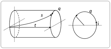
Figure 11 Complex time depicted on a cylindrical surface.

The cylindrical representation introduces intricacies, such as illustrating vectors on a contoured surface. For practicality, we often employ a flat representation of the cylinder, as in Figure 12. This flat representation demarcates boundaries on the imaginary time axis, dependent on the parameter $L_I$ , which signifies the extent of imaginary time. It's crucial that the flattening process preserves the total size of the imaginary time dimension equivalent to the $L_I$ parameter.

An alternative representation, shown in Figure 13, allows only positive values for imaginary time, reflecting the representation in Figure 12.

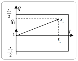
Figure 12 Flat projection of complex time.

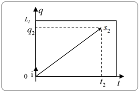
Figure 13 Representation of complex time with positive flattening.

This complex time representation can be paralleled with the operation of an old black and white TV, using a single electron beam to scan a luminescent screen. Each new image represents a new instance of real time, while the time taken by the beam to scan the entire screen equates to imaginary time.

In Figure 14, the top illustration uses dotted lines to denote scanning time, with each gap symbolizing the creation of a new image. Conversely, the bottom representation shows a complex plane derived by bending the line from the top graph, resembling the complex time diagrams in Figures 12 and 13.

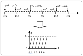
Figure 14 TV scan time represented as complex time.

Advantages of utilizing complex time

Exploring the use of imaginary time within a physical model might seem abstract, particularly as it's not directly observable. However, the complex digital time model proposed here offers several notable advantages:

1. String transformation: Complex time introduces the potential for point particles to spontaneously evolve into strings, arising from the collapse of the imaginary time dimension.
2. Alignment with string theories: Modern string theories often involve higher-dimensional frameworks, typically with a single time-related dimension. The inclusion of complex time, potentially as a wrapped dimension, offers symmetry and simplification in these models.
3. New perspective on cosmic inflation: The complex time model suggests that the early rapid expansion phase of the universe occurred solely within the imaginary time dimension growing, keeping real time static.
4. Understanding accelerated space expansion: Incorporating imaginary time progression helps explain the observed accelerated expansion of the universe, potentially negating the need for "dark energy."
5. Estimating the universe age and size: Calculating the length of imaginary time could provide a method to estimate the universe age and from it calculate the size of the universe.
6. Influence on physical constants: It's proposed that key physical constants might be influenced (growing) by the length of the imaginary time dimension.

These points are further detailed in the following sections, providing a comprehensive overview of the implications and benefits of incorporating complex time into current models.

Transformation of point particles into strings

In traditional physics, many models are predicated on point particles, which are presumed to be dimensionless. This concept simplifies the description of fundamental particles, however, it encounters difficulties, especially in situations where forces vary inversely with distance, leading to mathematical issues like division by zero during direct particle contact.

To address these complications, "string theories"⁵ have been proposed. These theories portray fundamental particles as strings, which can take the form of lines or membranes, offering a more robust framework. Yet, despite their potential, none, including the renowned M-theory,⁶ has yet to establish itself as a new paradigm or demonstrate practical application beyond theoretical constructs. This article posits that a key challenge in string theories is the absence of a clear mechanism for the transition from point particles in to strings. As point particles move through complex time, they naturally transform into strings due to the collapse of the imaginary time component. This change is universal, affecting all beings and instruments in the universe that are unable to perceive imaginary time, and so for then the imaginary time is always collapsed.

Figure 15 illustrates this transformation: A five-dimensional point particle (red dot) navigating complex time follows a dotted-line trajectory. Observers lacking the ability to perceive imaginary time would see this particle as a string (red line in Figure 15) that occupy the original particle path.

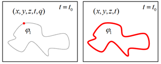
Figure 15 Transition of a point particle into a string through the lens of imaginary time.

Distribution of wrapped dimensions in space-time

Wrapped spatial dimensions are pivotal in string theory models.⁷ Often imperceptible to observers, these dimensions challenge the acceptance of such theories. For example, M-theory proposes eleven dimensions: three standard space, seven wrapped space, and one time dimension.

Introducing the Ulianov String Theory (UST),²⁴ this model perceives complex time as a wrapped dimension, forming a ten-dimensional space-time. UST incorporates three standard and three wrapped space dimensions, plus two standard and two wrapped time dimensions. This approach, aligning with dimensions in existing string theories, balances the distribution. Each normal dimension ($x, y, z, t, q$ ) pairs with a wrapped counterpart $(x,\overline{y},\overline{z},\overline{t},\overline{q}),$ simplifying analyses. It envisions wrapped dimensions as part of "sub-spaces" parallel to normal ones, separated by "time" or "space" walls, as shown in Figure 16.

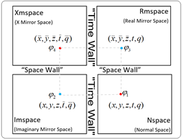
Figure 16 The ten-dimensional space-time model used in UST.

Exploring cosmic inflation

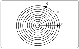
Cosmic inflation theory,⁹ introduced by Alan H. Guth in 1981, hypothesizes a swift exponential expansion of the universe shortly after the Big Bang.¹⁰ Despite its popularity, the theory faces criticism for its reliance on quantum physics without offering clear predictions, as highlighted by physicist Paul J. Steinhardt.¹¹ Central to this debate is the “inflaton” field, thought to amplify quantum fluctuations, leading to cosmic structures. However, this theory implies inconsistent inflationary endpoints across space, suggesting ongoing inflation in some regions. The complex time structure presents a novel approach, proposing uniform inflation irrespective of location or quantum fluctuations. This model, depicted in Figures 8, 9, and 17, posits that both space and time dimensions start with zero magnitude and size. The expansion of imaginary time initially forms concentric circles at the cylinder's base, shaping the complex time structure.

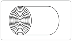
Figure 17 Illustration of the expanding imaginary time, forming the foundational base of the complex time cylinder.

As real time remains static, the complex time dimension expands until reaching a certain magnitude. The universe's expansion is linked to imaginary time progression, allowing for consistent growth even when real time is stagnant.

Figure 18 illustrates this concept, showing the universe's expansion as both blue (proposed model) and red (imaginary time expansion) curves. The difference in perceived expansion rates between observers aware and unaware of imaginary time is striking. To the latter, the universe appears to expand infinitely in an instant, while those understanding imaginary time see a gradual expansion.

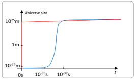
Figure 18 Dual representations of the universe's expansion trajectory.

This perspective suggests replacing the conventional cosmic inflation model with one that eliminates the need for an expansive field and resolves the expansion endpoint issue. In this model, the "Big Bang" becomes a more subdued "Small Bang," offering a more coherent explanation of the universe's early expansion and matter antimatter creation to made sphiral galaxies and supermassive antimatter black holes.

A comprehensive explanation of the space accelerated expansion 

This section models the interplay between space expansion and imaginary time extension.

Consider a two-dimensional space delineated over a sphere with radius $R_e$ , the total length of these space axes was given by:

$L_x=\text{ 2 }\pi R_e\text{ ; }{L}_y=\text{ 2 }\pi R_e$   (2)

As the sphere expands by one Planck length at each imaginary instant, linked to an "Imaginary Planck time," the radius $R_e$  expands at light speed:

$R_e =\text{ c }q$   (3)

Given the cyclic nature of imaginary time and the continuous growth of $R_e$ , it's pertinent to represent complex time using polar coordinates:

$s=p e^{ \alpha \text{ i}}$   (4)

Here, p signifies the magnitude of complex time, computed as:

$p=\sqrt{t^2+q^2}$   (5)

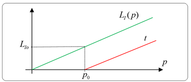
During the inflationary phase, dominated by complex time, consider the diagram shown in Figure 18. The extension of imaginary time steadily increases as:

$L_I\left(p\right)=2\pi p$   (6)

Presuming that, by the culmination of the imaginary time expansion, the complex time magnitude equals to $p_0$ , the length of imaginary time defined as $L_{I0}$  can be calculated as:

$L_{I0} = 2\pi p_0$   (7)

Final radius $R_{e0}$ can be inferred from equation (3), and the total imaginary time trajectory equals the combined area of circles in Figure 19, normalized with respect to Planck time ($T_P$ ):

$\begin{array}{l} R_{e0} = 2\pi {\left(\frac{ p_0^{}}{T_p}\right)}^2{L}_P\\ R_{e0} = \frac{2\pi \text{ c }{p}_0^2}{T_p}\end{array}$   (8)

Figure 19 Evolution of Complex Time in the Inflationary Phase.

Note that $p_0^{}$ is given in seconds and so $R_{e0}$ given in meters $(\frac{m}{s}{s}^2\frac{1}{s})$ but it value is related to one number of Panck distances.

By integrating Equation (7) into Equation (8):

$R_{e0} =\frac{\text{c }{L}_{I0}^2}{2\pi {\text{ T}}_p}$   (9)

Assuming consistent expansion rates for $L_{I0}$ and $R_e$ , Figure 20 illustrates imaginary time expansion (Equation 7) and real-time expansion (Equation 5) with zero angle in polar coordinates:

$t = p-p_0$   (10)

Figure 20 Illustration of the expansion of the lengths of imaginary and real time, dependent on the modulus of complex time.

Substituting from equation (7) into equation (10), we get:

$L_I =2\pi \left( p_0+t\right)$   (11)

As the $p_0^{}$ value is about ${10}_{}^{-30}$ seconds equation 11 can be simplified to:

$L_I =2\pi \text{ p }\cong 2\pi \text{ t}$   (12)

From Figure 20, we can deduce a generalized equation for the expansion of $R_e$ , which is defined at the point $p_0$ , in equation (8):

$\begin{array}{l}{R}_e\left(p\right)= \frac{2\pi c}{T_P}\underset{0}{\overset{p}{{\displaystyle \int }}}{L}_I\left(p\right)dp=\frac{2\pi c}{T_P}\underset{0}{\overset{p}{{\displaystyle \int }}}2\pi p dp\\ R_e\left(p\right)=\frac{4{\pi }^{2}c}{T_P}\frac{1}{2}{p}^2\end{array}$   (13)

$\begin{array}{l}{R}_e\left(p\right)=\frac{2{\pi }^{2}c{p}^2}{T_P}\\ R_e\left(p_0\right)= R_{e0}=\frac{2{\pi }^{2}c{p}_0^2}{T_P}\end{array}$   (14)

Note that equation (14) is the same equation (8) deduced by other way.

By substituting equation (11) into equation (13):

$\begin{array}{l}{R}_e\left(t\right) =\frac{2{\pi }^2\text{c}}{T_P} {(}^t\\ R_e\left(t\right)\cong \frac{2{\pi }^2\text{ c}}{T_P} t^2\end{array}$   (15)

With $R_e\left(t\right)$ given in number of Planck Length and ${\text{T}}_P$ is the Planck Time.

Finally, when substituting equation (2) into equation (15) and determining the spatial length $L_x$ as a function of real time:

$L_x\left(t\right)= \frac{\text{πc}}{T_P} t^2$   (16)

With $L_x\left(t\right)$ has it unit in meter but it value is relayed to a number of Planck Lengths. To obtain $L_x$ in meter we need multiply it by the value of Planck Length $(1.6 \times {10}^{-35})$

$\begin{array}{l}{L}_x\left(t\right)= \frac{\pi c }{T_P} L_P{t}^2\\ L_x\left(t\right)= \pi c^2{t}^2\end{array}$   (17)

Note that in equation (15) $L_x$ units seems given in $m^2$ but in fact the $c^2$ value in this equation is equal to 299792458²  but its unit is m/s².

Equation (15) shows that if we consider the complex time represented by a cylinder the imaginary time, expands linearly with real time, but the space length can be associated with the area of the section of the cylinder and its grown will be accelerated (proportional to $t^2$ ) to an observer in real time, aligning with cosmological observations without invoking dark energy for explanation. Using t equal to 13.8 billions of years ($4.35\times {10}^{17}s$ ) equation (15) given a space length of about $15\cdot 3\times {10}^{56}m$ , like the observable universe has only $8\cdot 1\times {10}^{26}m$ it is only a square root of the total length.

Determining the length of the imaginary time dimension

Earlier discussions provided a foundation for understanding time as a complex variable, emphasizing the significance of the imaginary time dimension, denoted as $L_I$ . The uniqueness of $L_I$ is underscored by its dynamic nature; it doesn't remain static but evolves continuously, compelling its evaluation at specific real-time junctures.

Before delving into the methodology to estimate $L_I$ , two pertinent questions emerge:

1. Without direct access to imaginary time, is an estimation of its length plausible?
2. If one could ascertain the length of imaginary time, what would be its physical interpretation?

At a glance, the answer to the first query seems negative. Analogously, it's akin to a cartoon character attempting to determine the computer's rendering time for its animation frames. In essence, without experiencing imaginary time firsthand, its quantification seems improbable.

However, certain scenarios offer a potential solution. Consider Figure 15, where a point particle transforms into a string. If this particle traverses at the speed of light, its length mirrors $L_I$ times the speed of light. This implies that estimating a particle's extension indirectly determines $L_I$ itself, a concept discussed in reference.¹⁶ Yet, this approach isn't devoid of pitfalls. The particle might loop multiple times, resulting in an underestimation of its actual length.

Another avenue is the extrapolation from Figure 20, where, under the assumption of a negligible $p_0$ , $L_I$ could be equated to the universe's age around 13.8 billion of  years. While the feasibility of identifying an imaginary time metric remains debatable, the question of its physical meaning persists. Terms like "imaginary year" or "imaginary second" initially seem nebulous. However, translating them to Planck time units offers clarity: 13.8 billion years equate to approximately 8.0x10⁶⁰ imaginary time units, that in fact define 8.0x10⁶⁰ "processing steps" to “draw” each particle that exist in our universe.

This exploration into the realm of complex and digital time offers a transformative perspective in understanding the cosmos. By integrating imaginary time as a complex and digital variable, new insights into the universe's creation and expansion are unveiled. This approach not only refines string theory but also elegantly explains the transition from point particles to strings. A notable outcome of this model is its ability to estimate the universe's age and size. Considering an $L_I$ value of approximately $8.0\times {10}^{60}$ units, our universe might span an astonishing $15.3\times {10}^{52}$  meters or $3.3\times {10}^{87}$ Planck lengths. Such a vast expanse, derived from the principles of complex time, underscores the potential of this theoretical framework in reshaping our cosmic understanding.

ANNEX 01 – Particles velocity’s in digital universes

The first aspect to be observed about  particle (or object or body) velocity's over any Digital Universe, is that in any digital universe, velocity is an emerging concept, which in fact does not exist within a time frame (associated to a 2D or 3D space), which always represents a set of objects stationary in space (with no defined velocity).

The notion of speed or velocity only arises when several frames are considered in sequence, but it is nothing more than an illusion.

Likewise, on a chess board we always see all pieces standing still in the chess board houses, and the occurrence of a new game move forces the creation of a copy of the board (in a new frame of space that can be associated to a new time), with all the pieces standing in the same place, with the exception of the piece to be moved which is copied in a new position.

So given two frames of space being considered distant from each other by a certain number of positions (which can be associated with a time interval). The average speed or velocity of a particle, can be defined by the relationship between the number of space houses that this particle jumped (from its position in the initial frame to the position in the final frame), divided by the distance that separates the frames in time, generating a metric of  number of houses jumped by number of moves, that can be associated with a value of meters per seconds.

So, when any object is moved in a artificial digital universe there are only two types of behaviour:

A - Continuous movement: In this kind of movement only two possibilities of movement can exist:

• The object stops in the same place (same $\left(x_0,y_0\right)$ 2D position or $\left(x_0,y_0,z_0\right)$  3D position) from one space-time frame (with $t=t_0$ ) to the next space-time frame (with $t=t_0+t_u$ );
• The object "jumps" from the 4D house $\left(x_0,y_0,z_0,t_0\right)$ to the neighboring 4D house, with six new 4D houses possibilities: $\left(x_0\pm d_u,y_0,z_0,t_0+t_u\right)$ or $\left(x_0,y_0\pm d_u,z_0,t_0+t_u\right)$  or  $\left(x_0,y_0,z_0\pm d_u,t_0+t_u\right);$

Were $t_u$ is a unitary time that separate two space frames and $d_u$  is a unitary distance between two neighbouring points in space. Note that in terms of one 4D space time stored inside of a 4D matrix the $t_u$  and $d_u$  values are unitary and given a unitary system representation, but it can be related to some real or virtual system and so given a specific value for $t_u$  and $d_u$  

This scheme allows only two speeds: zero speed and unitary speed (which is also the $d_u/t_u$ value, that represents the maximum continuous movement speed, associated with the light speed in a given Digital Universe).

For example the Minecraft game use 3D blocks with 1 meter of size to represent objects and distances inside of the game (That's why the objects in this game are square and have low resolution) so $d_u$ in the Minecraft universe is equal to 1 meter, and the game use about 30 frames per second and so $t_u$ = 1/30 seconds. On this way the light speed in the Minecraft universe is 30 m/s.

Now if we get the old pong game, where a ping-pong table is represented by the entire screen, the ping pong ball in one pixel a some $\left(x_{ball},y_{ball}\right)$ position. If we have a big screen with 0.5 meter of wide and containing, for example, 2000 points, the value of $d_u$  will be given by:

$d_u=0.5/2000=0.00025m$  or 0.25mm.

As this game also generate 30 images per second its $t_u$  is given by: $t_u=1/30$  seconds, in this case the speed of light is 30 pixels per second or only, 7.5mm per second, and so one ping pong ball using continuous movement will spend 66 seconds to cross the screen,Which would certainly make the game easy. But very boring. So in this case, the type of movement has to change and be faster than the speed of light.   

 B - Teleportation movement: In this case one particle can be stopped or jump several (N) houses at once (which represents a speed N times greater than the light speed ).

For example, in a chess game, pawns and the king have continuous movement, while knights, bishops, horses and queens is allowed to have teleportation movement, and can jump to distant squares, that can be considered superluminal speeds.

In the ping pong game for example if we want that the ping pong ball in one maximum velocity cross the screen size in two seconds, it needs move 2000 pixels in 60 frames given a need to jump 33 pixels in each new move (new frame). As this behaviour is very easy to be implemented, because we can drawn the ping pong ball in any place of the $\left(x,y\right)$ screen space in a new screen frame (representing a new time). So, in artificial digital universes the teleportation movement is normally available, unless some rule of the game only allows continuous movements, as is the case, for example, with the movement of a king and a top in a game of chess.

On the other hand, it is important to note that in a Digital Universe the minimum (not zero) speed, is given by the speed of light. So, speeds smaller than that of light cannot actually be implemented in DUs. In other words, the object cannot move a fraction of house or a fraction of the unitary distance, like a pawn in a chess game cannot move a half of one house. Then, to simulate a speed smaller than the light speed the object must remain stationary for a certain time (maintain the same $\left(x,y,z\right)$ position in some number of space frames sequences), then make a Jump at the light speed (jump to some neighbour house). Thus, for example, if the object remains stationary for 9 frames and moves with unit speed during one frame. The average speed will be equal to 0.1 house per frame or 10% of the light speed.

ANNEX 02 – Is it really impossible travel faster than light?

The fact is that we live in a digital space-time, where there are only 2 speeds: zero speed and the speed of light.

It's like a king moving on a chessboard, he can stay still or jump to a square.

Einstein's Special Theory of Relativity implies that the particle must choose to travel in time or travel in space.

Thus, when she jumps through space at the speed of light, she does not move in time (she does not "live" a Planck time-time frame) and when she jumps through time (the speed of light in time), she does not travel in space.

In this way, a body moving at 50% the speed of light implies that it is one time frame still and one time frame jumping at the speed of light (one Planck distance per Planck time) so it too will " skip" a time frame and live the next time frame (like a cinema film with black images inserted between every 2 normal images - which doubles the projection time) and thus, the time for it will be dilated by a factor (1–0.5²)^0.5 = 0.866 of "time speed" and time dilation of 1.15 (losing a time frame in every 2 seems to imply a time speed of 50% but it is a vector sum and thus generates 86.6 %).

If, for example, a billiard ball moves on a table at 1 m per second, this means that it jumps at the speed of light for a Planck time (advances a Planck distance) after which it stays 299,792,457 Planck times stationary, on average its speed will be:

$V_{mean}=\frac{c+0}{299792457+1}=1m/s.$

The ball repeats the cycle very quickly (5.56077x 10^⁵¹ times per second) so we see that they move continuously at 1 m per second, in the same way that we think that a film on the screen is continuous (above 20 frames per second ) when they are just sequences of frozen images.

This also implies that every 299792457 time frames the ball will miss one. So there will be a "time velocity" equal to 99.9999997% (time dilation of 1.000000003).

So, it makes no sense to ask why light moves at the speed of light or if a body can move at the light speed because the light speed of is the only non-zero velocity that exists in our universe.

To continuously jump in space (100% of the speed of light) the body would have to freeze in time, so it can jump 999,999,999 times in space and 1 time in the time and then it will have 0.999999999 of the light speed but its time will be a super frozen temporal speed of 0.00005 and temporal dilation of 20,000. It can also jump 999,999,999,999 times in space and 1 time in time and so he will have 0.999999999999 of the speed of light but his time will be frozen, with temporal speed of 0.000001 and temporal dilation of 10,000,000.

At first, it don't has a limit, and the temporal speed can be absurdly slow, like that in one second of the body time 10 billion years pass in the universe and then the body speed is almost equal to the light speed.

It is worth remembering that when a body skips one time frame, 2 copies of it exist at the same time (in the frame that be frozen when travel in space) and thus its mass value (average mass value at the time in which the body exists) increases, being inversely proportional to the temporal speed. So, a body with a temporal speed of 0.1 will have a mass 10 times greater (as there will be 10 copies of the same body in each time frame in which it exists)

Thus, in the example above, for a temporal speed of 0.00005, the mass of the body will be 20,000 times greater, as there will be 20 thousand copies of the same body in each time frame, displaced one to another by a Planck distance.

At first, a body does not notice the existence of these copies in the same time frame because when moving at low speed, they make jumps at the speed of light and then remain still for a short cycle. In this case there will be moments (when the body jumps at light speed) two copies of the body occupying the same place in space (displaced by a Planck distance), but the body does not feel this.

So, if you don't feel two copies, for 87% of the speed of light (3 copies) or 99% of the speed of light (7 copies) the same thing will happen: the copies don't interfere, it just gets heavier.

None.

None.

1. Einstein A. (1920). Relativity: The Special and General Theory. H. Holt and Company. 1920.
2. Adler R, Bazin M, Schiffer M. Introduction to General Relativity. McGraw–Hill New York. 1975.
3. Klein MJ. Max Planck and the Beginnings of Quantum Theory. Archive for History of Exact Sciences. 1962;459–479.
4. Ulianov PY, Freeman AG. Small Bang Model. A New Model to Explain the Origin of Our Universe. Global Journal of Physics. 2015;3(1).
5. Hawking S. A Brief History of Time. Bantam Books. 1998.
6. Planck M. Über irreversible Strahlungsvorgänge. Sitzungsberichte der Königlich Preußischen Akademie der Wissenschaften, 1899;440–480.
7. Wikipedia. Shrek.
8. Escher MC. Gravura Mãos Desenhando.
9. Green M, Schwarz J, Witten E. Superstring theory. Cambridge University Press. 1987.
10. Greene B. The Elegant universe: Superstrings, Hidden Dimensions, and the Quest for the Ultimate Theory. W.W. Norton & Company. 2003.
11. Green MB, Schwarz JH. Anomaly cancellations in supersymmetric D=10 gauge theory and superstring theory. Physics Letters B. 1984;149(1–3):117–122.
12. Guth AH. Inflationary universe: A possible solution to the horizon and flatness problems. Physical Review D. 1981;23(2):347.
13. Alpher RA, Bethe H, Gamow G. The origin of chemical elements. Physical Review. 1948;73(7):803.
14. Steibhardt PJ. The Inflation Debate. Is the theory at the heart of modern cosmology deeply flawed? Scientific American Magazine. 2011.
15. Koke S, Grebing C, Frei H, et al. Direct frequency comb synthesis with arbitrary offset and shot–noise–limited phase noise. Nature Photonics. 2010.
16. Ulianov PY. Small Bang Creating a Universe from Nothing. UFSC, Florianopolis. 2002.
17. Ulianov PY. Spacetime Dipole Wave Pressure And Black Holes A New Way To Obtain The Schwarzschild Metric, Without Using General Relativity Field Equations. Asian Journal of Mathematics And Physics Volume. 2013;2013(1):15.
18. Ulianov PY. An alternative to the Higgs field mass generation mechanism based on a dipole wave pressure model. Asian Journal of Mathematics and Physics. 2013;2013(1):7.
19. Ulianov PY, Freeman AG. Small bang model. A new model to explain the origin of our universe. Global Journal of Physics. 2015;3(1):6.
20. Freeman AG, Ulianov PY. The small bang model – a new explanation for dark matter based on antimatter super massive black holes. Journal of Modern Physics. 2015;3(1):150–164.
21. Ulianov PY, Negreiros JP. Does the value of Planck time vary in a black hole event horizon? A new way to unify general relativity and quantum mechanics. Global Journal of Physics. 2015;3(1):165–171.
22. Ulianov PY. Breaking the Paradigm of Negative Mass: Why Newton’s Second Law Needs to Be Modified to Enable Newton’s Gravitational Law to Deal with Antimatter. Global Journal of Physics. 2016;4(1):6.
23. Ulianov PY, Mei X, Yu P. Was LIGO’s Gravitational Wave Detection a False Alarm? Journal of Modern Physics. 2016;7(14):1845.
24. Ulianov PY. Ulianov string theory a new representation for fundamental particles. Journal of Modern Physics. 2018;2(1):77–118.
25. Ulianov PY. Ulianov Sphere Network–A Digital Model for Representation of Non–Euclidean Spaces. Curr Res Stat Math. 2023;2(1):55–69.
26. Ulianov PY. How can we observe waves without seeing the ocean? The Witte–Ulianov Time Interferometer: A Gravitational–Wave Detector Without a Lower Frequency Limit. Curr Res Stat Math. 2023;2(1);44–54.
27. Ulianov PY. Antimatter Enigma Solved: Astronomical Data Allows Identification of 77 Supermassive Antimatter Black Holes and 23 Antimatter Galaxies. 2023.
28. Ulianov PY. Ulianov Perfect Liquid Model Explaining why Matter Repels Antimatter. 2023.
29. Ulianov PY. 49 Paradogmas that Will be Broken by the Ulianov Theory. 2023.
30. Ulianov PY. A Comprehensive Overview of the Ulianov Theory. 2023.