On levy-walk model for correlations in spatial galaxy distribution

doi:10.15406/paij.2019.03.00162

eISSN: 2576-4543

Physics & Astronomy International Journal

Mini Review Volume 3 Issue 2

On levy-walk model for correlations in spatial galaxy distribution

VV Uchaikin

Verify Captcha

Regret for the inconvenience: we are taking measures to prevent fraudulent form submissions by extractors and page crawlers. Please type the correct Captcha word to see email ID.

Ulyanovsk State University, 42 Lev Tolstoy Str., Ulyanovsk 432700, Russia

Correspondence: VV Uchaikin, Ulyanovsk State University, 42 Lev Tolstoy Str., Ulyanovsk 432700, Russia

Received: March 14, 2019 | Published: March 29, 2019

Citation: Uchaikin VV. On levy-walk model for correlations in spatial galaxy distribution. Phys Astron Int J. 2019;3(2):82-88. DOI: 10.15406/paij.2019.03.00162

Download PDF

Abstract

The model of stochastic fractal is briefly described, basic results regarding properties of spatial structures with long-range correlations of power-law type are reviewed, and some applications to galaxy distribution in the Universe are discussed.

Introduction

One of important problems complicating the extraction of information from cosmological surveys, is necessity to supplement observational data subtracted of foreground or for some (i.e. technical) reasons removed from the survey. This particularly affects the extraction of information from the largest observable scales. Maximum-likelihood estimators are not quite applicable for reconstructing the full-sky because of non-Caussian character of observed matter distribution. To solve this problem, many authors modify implementations of such estimators which are robust to the leakage of contaminants from within masked regions. The trouble arises from the need to satisfy the cosmological principle of an arbitrary choice of the reference frame and long-distant correlations in spatial galaxy distribution observed. We are going to discuss here one а such approach and to show some results of its application. The discussion about homogeneity (or inhomogeneity) of the large-scale visible matter distribution in the Universe is attracting the attention of both the astronomers and theoreticians of cosmology.^1–⁴ In recent years the more complete and deeper galaxy surveys become available,^5,⁶ however, this does not eliminate the question about fractality of the large-scale structure. The fractal concept, introduced by Mandelbrot,⁷ applied to the galaxy distribution means the presence of the overdence regions and voids extending to all scales, at least to those could be reached by now. Mathematically, it formulates as

$N (R) \propto R^{D}$ (1)

for the ensemle averaged number of galaxies inside a sphere of radius R centered at any galaxy, D is the fractal dimension. Such a relation naturally originates from the model of self-similar ( hierarchical clustering.³ The aim of this work is not to prove or disapprove the fractality of the matter distribution in the Universe but only to deduce some conclusions about statistical properties of the structures with the long-range correlations of power type. The paper is organized as follows: Section I deals with the power spectrum being the Fourier transformation of two-point correlation function found in the galaxy distribution. From approximation of the real galaxy power spectrum it follows that galaxy distribution can be simulated within the frame of random walk model (Section II). Section III concerns the cosmological monopole and dipole which are the characteristics of large-scale homogeneity and isotropy. Here is also present the distribution of gravitational force magnitude (Holtsmark distribution). Section IV presents the distribution of number of points inside the spherical cells in the stochastic fractal model. In Section V the question about the global mass density of the fractal Universe is investigated with the empirical distribution density over masses adopted. In Section VI the ergodic problem in observational cosmology is discussed.

Power spectrum

The important statistical characteristic of the large-scale structure of the Universe is the two-point spatial galaxy correlation function,¹ which determines the joint probability

$δ P = n^{2} [1 + ξ (r)] δ V_{1} δ V_{2}$

to find two galaxies in volumes $δ V_{1}$ and $δ V_{2},$ placed at the distance $r = |x_{2} - x_{1}|$ from each other ( $n$ is the mean galaxy number per unite volume, i.e. the concentration). According to the assumption about homogeneity and isotropy of matter distribution in the Universe the mean galaxy number density $n$ should not depend on coordinates and $ξ (r)$ depends only on distance between the points chosen. Instead of $ξ (r)$ it is often used its Fourier transformation $P (k)$ called power spectrum¹

$n P (k) = V^{- 1} \int^{} ξ (r) e^{i k . r} d^{3} r,$ (2)

$ξ (r) = (V / 8 π^{3}) \int^{} P (r) e^{- i k r} d^{3} r .$ (3)

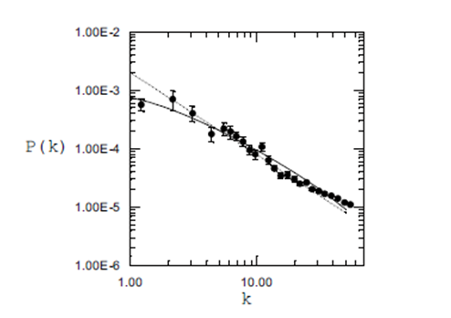
Figure 1 shows the power spectrum obtained from from the Lick Observatory catalog of Shane and Wirtanen,^8,⁹ where $k$ is expressed in units of “waves per box", physical wavelengths are $λ = 260 h^{- 1} M p c / k .$ There exists several approximations of power spectrum. The most simple of them is

$P (k) = A k^{γ}$ (4)

with $A$ being the amplitude of the spectrum and $γ \in (- 3, 0)$ in order to allow for the convergence of the integral of $P (k)$ at large wavelength. The value $γ = 1$ for the spectral index corresponds to the scale-free Harrison–Zel’dovich spectrum¹⁰ that describes the fluctuations generated in the framework of the canonical inflationary scenario.^11–¹³ Substituting (4) into (3), we get

$ξ (r) = (A V / 2 π^{2}) \frac{Γ (γ + 3)}{γ + 2} sin [\frac{(γ + 2) π}{2}] r^{- (3 + γ)} .$

Figure 1 Power spectrum P(k) (dots with error bars). The solid curve is approximate formula for $α = 1.5,$ , c = 0.018, $A = 10^{- 5}$ and q = 0.99. The dashed curve corresponds to the law $P (k) ~ k^{- 1.41}$ .

Thus, the detected power law shape for the correlation function $ξ (r) ~ r^{- α}, α ~ 1.8,$

turns into a constant logarithmic slope of the power spectrum with spectral index $γ = 3 - α$ at least at scales $r ? 10 h^{(- 1)} M p c [1, 14] :$

$P (k) = A k^{- 3 + α} .$

Here the exponent $a$ is equivalent to the fractal dimension $D$ . As one can see from Figure 1, the formula is in agreement with observed results in the region $3 \leq k \leq 30,$ but it may be improved in the region of small values of $k$ which affects the $ξ (r)$ at large distances. Obviously, there are many appropriate representations of it, but one of them leads us to a very useful and significant analogy:

$P (k) = A \frac{e^{- {(c k)}^{α}}}{1 - q e^{- {(c k)}^{α}}},$ (5)

where $c > 0$ and $0 \leq q \leq 1$ can be chosen in appropriate way (see Figure 1). The point is that the inverse Fourier transformation of expression (5) leads to the integral equation

$ξ (r) = A V p (r / c^{3}) + (q / c^{3}) \int^{} ξ (|x - x'|) p (x' / c) d^{3} x',$ (6)

where

$p (x) = \frac{1}{8 π^{3}} \int^{} e^{- i k . x - k^{α}} d^{3} k, k = |k| .$ (7)

The equation obtained is one form of the Ornstein-Zernike equation¹⁷ and can be used to clear up the relationship between statistical mechanics and the concepts under consideration. On the other hand, this equation leads us directly to the random walks model as a tool for construction of random point distribution with given correlations.

Random walk model

Let us consider the integral equation

$g (x) = p (x) + q \int^{} g (x - x') p (x') d^{3} x',$ (8)

so that

$ξ (r) = (A V / c^{3}) g (x), r = c |x| .$

The positive function $g (x)$ can be interpreted as a density of collisions of some particle starting its moving at the origin and performing the first collision in $d x'$ with probability $p (x') d^{3} x'$ where it stops with the probability $1 - q$ or performs the next jump into $d x''$ with the probability $q p (x^{″} - x^{'}) d^{3} x^{″},$ and so forth. So in this way of interpretation the points of collisions are positions of galaxies considered to be the point-like objects. The random walk model applied to simulation of galaxy distribution was firstly proposed by B.Mandelbrot.⁷ In his version the transition probability has the form of the pure power law $p (x) α r^{(- ?)} .$

The integral

$\int^{} g (x) d^{3} x = 1 / (1 - q), q < 1,$ (9)

gives the mean number of all collisions of the particle including the final one, and the function $g (x)$ itself can be expressed by its Neumann’s series expansion

$g (x) = \sum_{j = 1}^{\infty} q^{j - 1} p_{j} (x),$ (10)

where

$p_{1} (x) \equiv p (x)$ (11)

and

$p_{j + 1} (x) = \int^{} p_{j} (x - x') p (x') d^{3} x'$ (12)

is the multiple convolution of the distribution density $p (x)$ . Here it should be noted that the probability density (7) with $α \in (0, 2]$ belongs to the set of symmetrical three-dimensional stable distributions.¹⁶ One of them, with $α = 2,$ is the famous Gauss’ law, but the others are utilized by physicists rarely enough, although in probability theory they play the same role in the problem of summation of independent random values with infinite variance. Generally, the densities are not expressed in terms of elementary functions and must be calculated numerically. Two properties of the laws are very important for the problem. First, the stable density with $α < 2$ has an inverse power tail at large distances,

$p (x) ~ \frac{1}{2 π^{2}} Γ (2 + α) s i n (\frac{π a}{2}) r^{(- ? - 3)},$

and second, multiple convolutions of this density are expressed in terms of original density with rescaled argument:

$p_{j} (x) = \frac{1}{8 π^{3}} \int^{} e^{- i k . x - j k^{α}} d^{3} k = j^{- 3 / α} p (x j^{- 1 / α}) .$

Now we consider an infinite set of independent trajectories of such kind starting from different random points of birth distributed by Poisson uniform law with the mean density $n_{0} .$ Using the generating functional technique, we obtained in our work,¹⁸ that in this case

$g (x) = \frac{n c^{3}}{2 q} ξ (r),$ (13)

where

$n = \frac{n_{0}}{1 - q} .$

Remark. As one can see from the latter expression, passage to infinitely long trajectories (q to1) саn be realized only in accompaniment with rarifying seed distribution $(n_{0} to 0) .$ is the density of all points of collisions. Moreover, correlation functions of all orders $ξ_{m},$ $m > 2,$ are expressed through $ξ_{2} (r) \equiv ξ (r)$ as follows

$ξ_{m} (r_{1}, \dots, r_{m}) ≐ m! Q_{m} ξ_{12} \dots ξ_{m - 1, m}$

where

$ξ_{i j} = ξ (|x_{i} - x_{j}|), Q_{m} = {(1 / 2)}^{m - 2},$

And $≐$ means the symmetryzation operator.Thus, three-point and four-point correlation functions are of the forms

$ξ_{3} (r_{1}, r_{2}, r_{3}) = Q_{3} \{ξ_{12} ξ_{23} + ξ_{21} ξ_{13} + ξ_{13} ξ_{32}\} ≐ Q_{3} \{ξ_{12} ξ_{23} + c y c l . (3 t e r m s)\}$ (14)

and

$ξ_{4}^{[q]} (1, 2, 3, 4) ≐ Q_{4} \{ξ_{12} ξ_{23} ξ_{34} + c y c l . (12 t e r m s)\} .$ (15)

It is well known that the observed function $ξ_{3}$ for the galaxy distribution, denoted usually as $η,$ has really the form (14), but the factor $Q_{3}^{obs}$ is in the neighborhood of 1 $(0.8 \leq Q_{3}^{obs} \leq 1.3)$ . It is noted that the lower limit may be even less than indicated.¹ The observed function $ξ_{4}$ denoted by $ζ,$ contains additional terms like $ξ_{12} ξ_{13} ξ_{14}$ being absent in (15). Thus the model dealing with non-branching trajectories doesn’t give exhaustive description of all statistical properties of galaxies distribution although the two-point function (13) is in good agreement with observed data.^1–¹⁵ Possibly, the way out of this situation can be found in involving the branching trajectories into the model. In this case a random number of secondary particles arises in every collision and then all of them move independently of each other.

Cosmological monopole and dipole

The current value of the average mass density in the Universe is estimated as

$ρ_{0} = 1.88 \cdot 10^{- 29} Ω_{0} h^{2} {g cm}^{- 3},$

Where $h$ is the dimensionless parameter connected with the uncertainty of Hubble’s constant $H$ ,

$0.5 \leq h \leq 1,$

And $Ω_{0}$ stands for the cosmological density parameter. It is customary to consider that the modern value of the parameter lies in the interval

$0.03 \leq Ω_{0} \leq 1.$

As a first approximation the Universe looks like a uniform Hubble flow with the relative velocity

$v = H (t) r,$

forming the background for observations of peculiar motions of galaxies. Assuming that gravitational instability is the cause of the observed peculiar motions, these local deviations from a uniform Hubble flow provide a powerful tool for studying the local mass distribution and hence estimating the cosmological parameter $Ω_{0}$ .

Using linear perturbation theory, the peculiar velocity $v_{p}$ can be related to the peculiar acceleration $g$ via

$v_{p} \propto w (Ω_{0}) g,$

Where $w (Ω_{0})$ measures the logarithmic rate of growth of the mass fluctuation at the present epoch.¹ Calculations yield¹⁹

$v_{p} = d_{conv} \frac{Ω_{0}^{0.6}}{3 b} \frac{D}{M} (\leq d_{conv}),$

Where $M$ and $D$ are the monopole and dipole moments obtained from observations via relations

$M = \frac{1}{4 π} \sum_{i = 1}^{n} \frac{1}{ϕ (r_{i})} \frac{1}{r_{i}^{2}}$

and

$D = \frac{3}{4 π} \sum_{i = 1}^{n} \frac{1}{ϕ (r_{i})} \frac{x_{i}}{r_{i}^{3}} .$

Here $x_{i}$ are positions of galaxies, $ϕ (x_{i})$ is a selection function to take into account the fact that at different distances we sample different portions of the luminosity function, $d_{c o n v}$ is the depth at which the dipole converges to its final value and $b$ is the bias factor that relates galaxy to mass overdensities. The $Ω_{0}^{0.6}$ factor comes in when one uses the theory of linear gravitational instability to relate the peculiar velocity to the gravitational acceleration.¹

Supposing for simplicity

$M_{R} = \frac{1}{4 π} \sum_{i} \frac{1}{r_{i}^{2}} 1 (x_{i}; U_{R})$

and

$D_{R} = \frac{3}{4 π} \sum_{i} \frac{x_{i}}{r_{i}^{3}} 1 (x_{i}; U_{R}),$

Where $1 (x_{i}; U_{R})$ is the indicator function of the ball $U_{R}$ with radius $R$ centered at the observation point x=0, and assuming uncorrelated homogeneous Poisson distribution of galaxies (q to 1, $n_{0} to 0) .,$ one can write the joint characteristic function

$f (q, k) = e^{i q M_{R} + k_{^{.}} D_{R}}$

in the form:

$f (q, k) = exp \{- n \int_{U_{R}} [1 - e^{i (q M_{R} + k . D_{R})}] d^{3} x\} .$

Putting here $q = 0$ and then $R \to \infty,$ we arrive at the known Holtsmark distribution for $D,$ and in the case $k = 0$ we obtain the one-sided one-dimensional stable distribution with $α = 3 / 2,$ for $M_{R} - E M_{R}$ . Note that the fact

$lim_{R \to \infty} M_{R} = \infty$

is known as Olbers’ paradox and unfortunately its solution is obtained without using stable laws (see [20]).²⁰ A number of authors analyze the dependence of observed cosmological dipole $D_{R}$ on $R$ interpreting its saturation as an evidence for homogeneity of the Universe, some authors interpret the saturation as an evidence for isotropy of the Universe. For a complete review of this discussion we refer the reader to works.^3–²³ In any case this quantity bears a direct relation to the Cosmological Principle which can be formulated in the following way: “Except for local irregularities, the Universe presents the same aspect, from whatever point it is observed”.²⁴ The dependence $D_{R}$ on $R$ for some fractal models of the Universe has been investigated in the works.^21–²⁵ We performed Monte-Karlo simulations of the distribution of the absolute value of summarized gravitational force of galaxies in two cases: homogeneous Poisson galaxy distribution (in result we get Holtsmark distribution) and in the case of fractal galaxy distribution, which we obtain using Mandelbrot trajectory. As one can see from the Figure 2 in fractal case the distribution is greatly wider than in Poisson case.

Figure 2 The distribution of absolute value of gravitational force. (a) – Poisson galaxy distribution, (b) – fractal galaxy distribution with D = 1.5

Cell-count distribution for the fractal Universe

The characteristics of the fractal distribution is the count of the number of galaxies in the spherical volume of radius $R$ . The average value obeys the relation (1). The numerical calculations performed in,²⁶ yield the following distribution of $N (R)$ for the stochastic fractal model:

$P \{N (R) = n\} ~ \frac{1}{N (R)} Ψ (\frac{n}{N (R)})$ (16)

where

$Ψ (z) = \frac{1}{Γ (λ)} λ^{λ} z^{λ - 1} e^{- λ z}$ (17)

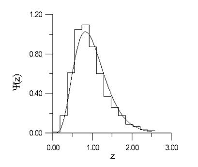
is the gamma-distribution. Distributions of $N (R)$ called cell-count distributions are obtained from galaxy catalogs by means of not very reliable procedure. Nevertheless it is interesting to compare the fractal cell-count distribution (4) with observed data. To do this we have taken the Lick sample data presented in the paper [27]. Computing $〈 N (R) 〉$ we have found $Ψ^{obs} (z)$ and calculation of $〈 N^{2} (R) 〉$ has given us a possibility to find the parameter $λ$ in approximation formula (17). The two distributions presented in Figure 3 have turned out to be very close to each other.

Figure 3 Distributions $Ψ (z)$ (solid curve) and $Ψ^{obs} (z)$ (step diagram).

Global mass density for the fractal universe

One of important parameters characterizing models of the Universe is the global mass density

$ρ = \underset{R \to \infty}{l i m} [M (R) / V (R)],$ (18)

Where $M (R)$ is the total mass within a sphere of radius $R$ and $V (R)$ is the volume of the sphere. For models being homogeneous (at least on large scales) this limit exists and is not zero. Let us see what kind of results one can get for fractal models. At first we consider the deterministic fractal described in the paper.³ Starting from a point occupied by an object and counting how many objects are present within a volume characterized by a certain length scale, we get $N_{0}$ pointlike objects within a radius $R_{0},$ $N_{1} = q N_{0}$ objects within a radius $R_{1} = k R_{0},$

$N_{2} = q N_{1} = q^{2} N_{0}$ objects within $R_{2} = k R_{1} = k^{2} R_{0}$ and so on. In general we have

$N_{n} = q^{n} N_{0}$ (19)

and

$R_{n} = k^{n} R_{0},$ (20)

Where $q$ and $k$ are constants. By taking the logarithm of equations (19) and (20) and dividing one by the other we get

$N_{n} = C R_{n}^{D}$ (21)

with

$C = N_{0} R_{0}^{- D},$

$D = \frac{l n q}{l n k},$

Where $C$ is a prefactor of proportionality related to the lower cutoffs $N_{0}$ and $R_{0}$ of the fractal system, that is, the inner limit where the fractal system ends, and $D$ is the fractal dimension $(D < 3)$ . If we smooth out the point structure we get the continuum limit of equation (21)

$N (R) = C R^{D} .$ (22)

Supposing that all the objects have the same mass , we get

$ρ (R) \equiv M (R) / V (R) = [3 m C / (4 π)] R^{- γ}, γ = 3 - D .$

As one can see from here,

$ρ = lim_{R \to \infty} ρ (R) = 0,$ (23)

for the fractal structure. This fact is known as the third postulate of the pure hierarchy fractal conception: "for a pure hierarchy the global mass density is zero everywhere".⁴ The situation stays the same if masses $m_{i}$ are independent identically distributed random variables with $E m_{i} = 〈 m 〉 < \infty :$

$〈 ρ (R) 〉 \equiv 〈 M (R) / V (R) 〉 = [3 〈 m 〉 C / (4 π)] R^{- γ} .$

However, astronomical observations show that in a very large range of masses the probability density $p (m)$ has the form

$p (m) = β A m^{- β - 1}, 0 < m_{0} < m,$ (24)

where $β$ is less than 1.²⁸ We will suppose further that (17) holds true for all $m > m_{0} .$ Introducing the random value

$ρ (R) = \sum_{i = 1}^{N (R)} m_{i} / V (R) = [3 / (4 π)] R^{- 3} \sum_{i = 1}^{N (R)} m_{i},$ (25)

one can transform the problem of finding $〈 ρ 〉$ which is infinite now into the problem of investigation of the distribution of the random variable (25). In the case $β < 1,$ the distribution (24) belongs to the domain of normal attraction of a one-dimensional standardized stable law $p (x; β)$ with the characteristic exponent $β,$ so that

$Prob \{\sum_{i = 1}^{N} m_{i} / b_{N} < x\} \Rightarrow G (x; β), N \to \infty$ (26)

Where $G (x; β)$ is the distribution function and

$b_{N} = b_{1} N^{1 / β}$ (27)

and

$b_{1} = {[A (1 - β) cos (β π / 2)]}^{1 / β} .$

Denoting the probability density of the random variable (25) by $p_{ρ} (x; R)$ and using (26), one can obtain the following asymptotical expression for large values of $N (R) :$

$p_{ρ} (x; R) ~ [4 π R^{3} / (3 b_{N (R)})] p (4 π R^{3} x / [3 b_{N (R)}]; β),$

$N (R) \to \infty .$ (28)

Substituting (22) into (27) and inserting result into (28), we get

$p_{ρ} (x; R) ~ Q R^{3 - D / β} p (Q R^{3 - D / β} x; β),$ (29)

$R \to \infty,$

where

$Q = 4 π / (3 b_{1} C^{1 / β}) .$

As one can see from (28), the probability density of the random conditional mass density has a nondegenerated limit by $R \to \infty$ for $β = D / 3 :$

$p_{ρ} (x; R) \underset{R \to \infty}{\to} p_{ρ} (x) \equiv Q p (Q x; β),$ (30)

$β = D / 3.$

The aggregate considered above seems too artificial to be used as a model of mass distribution in the Universe. The stochastic fractal described in Sec. II is more appropriate for this purpose. In this case

$p_{ρ} (x; R) = 〈 p_{ρ} (x; R, N (R)) 〉$

Where $p_{ρ} (x; R, N (R))$ is the conditional density by a fixed value $N (R)$ and $〈 \dots 〉$ means here averaging over the random variable distributed according the law

$P \{N (R) = n\} ~ \frac{1}{〈 N (R) 〉} Ψ_{D} (\frac{n}{〈 N (R) 〉}),$

With

$Ψ_{D} (z) = \frac{λ^{λ} z^{λ - 1}}{Γ (λ)} e^{- λ z}$ (31)

Taking into account (29), we get

$p_{ρ} (x; R) ~ Q R^{3 - D / β} \int_{0}^{\infty} z^{- 1 / β} p (Q R^{3 - D / β} x z^{- 1 / β}; β) Ψ_{D} (z) d z .$

Therefore the nondegenerated limit of the distribution of $ρ$ exists under condition $β = D / 3$ again:

$p_{ρ} (x) = Q \int_{0}^{\infty} z^{- \frac{1}{β}} p (Q x z^{- \frac{1}{β}}; β) Ψ_{D} (z) d z .$

Rescaling the independent variable $Q x \to x$ and substituting here (31) we arrive the following expression

$p_{ρ} (x) = {[Γ (λ)]}^{- 1} λ^{λ} \int_{0}^{\infty} z^{λ - 1 - 1 / β} p (x z^{- 1 / β}; β) e^{- λ z} d z .$ (32)

It is easy to check, that this result obeys normalization

$\int_{0}^{\infty} p_{ρ} (x) d x = .1.$

Astronomical observations show that $D \approx 1.16 \div 1.40.$ .²³ Taking for the sake of simplicity $D = 1.5,$ we get the value

$β = 0.5,$

which coincides approximately with

$β_{o b s} = 0.5 \div 0.6$

obtained from luminosity observations.¹⁴ In this case one can use an explicit form of the stable density

$p (x; 1 / 2) = \frac{1}{\sqrt{2 π}} x^{- 3 / 2} e^{- \frac{1}{2 x}},$

so (32) takes the form

$p_{ρ} (x) = \frac{λ^{λ} x^{λ / 2 - 1}}{\sqrt{2 π} Γ (λ)} \int_{0}^{\infty} t^{\frac{λ - 3}{2}} e^{- λ {(x / t)}^{1 / 2}} e^{- \frac{1}{2 t}} d t ..$

Using formula (3.462) from the book,²⁹ one can rewrite the result in the form

$p_{ρ} (x) = \frac{2 λ^{λ} x^{λ / 2 - 1}}{\sqrt{π} Γ (λ)} Γ (λ + 1) e^{(λ^{2} x) / 4} D_{- (λ + 1)} (λ \sqrt{x})$

Where $D (x)$ is the parabolic cylinder function and $λ = 1.5$ for a single fractal and $λ = 3$ for a fractal which is a paired Mandelbrot trajectory.²⁶ The graphs of $p_{ρ} (x)$ for deterministic fractal, single and coupled stochastic fractals are represented in Figure 4. As we can see the distributions are broad enough with the same asymptotics $x^{- 3 / 2}$ .

Figure 4The Distribution of GMD in the case of deterministic fractal (solid line), single Mandelbrot trajectory (dashed line) and paired Mandelbrot trajectory (dotted line).

Ergodic problem

Among the other problems concerning the large scale structure of the Universe the special place is taken by the some hypotheses which are, maybe implicitly, underlying the standard correlation function analysis. Note that all the descriptive statistics used for analyzing the large-scale structure neglect the curvature of the space and expansion of the Universe, i.e. these statistics work in Euclidean space. Also the next fact is neglected: the galaxies are seen in the past light cone but not in the fixed moment of cosmological time. This is a good approximation since the most available data is obtained from the small part of Hubble distance $c H^{(- 1)}$ .¹ The Fair Sample Hypothesis is also implied, it states:

it is quite reasonable to treat those parts of the Universe which are sufficiently separated from each other as independent realizations of the one and the same physical process;
within the limits of the visible Universe there are many independent samples which can be gathered into approximate statistical ensemble;
the turning does not change the values averaged over ensemble;

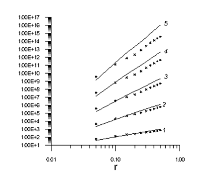
Under such assumptions they usually perform statistical analysis of galaxy distribution. However, in the light of fractal approach to the large scale structure, more attention should be paid to the newly arisen problem which we can call Cosmological Ergodic Problem induced by Ergodic Hypothesis.³⁰ Astronomical observations probe only the spatial distribution in one realization of some physical process. Theory, on the other hand, specifies the probability distribution over an ensemble. For homogeneous random fields Ergodic Hypothesis states: ensemble averages equal spatial averages taken over one realization of the random field. Note that, in contrast with the custom of statistical mechanics, this Ergodic Hypothesis refers to the spatial distribution of the random field at a fixed time rather than to the time evolution of the system. Essentially, the Ergodic Hypothesis requires spatial correlations to decay sufficiently rapidly with increasing the separation so that there exist many statistically independent volumes in one realization. This fact is usually implied when statistically treating the large-scale structure, but is it a real fact ? Can we suppose the available surveys to be big enough to provide us with a certain confidence about presence of independent samples? Anyway, leaving apart the discussion about actual fractality of the Universe³ the conclusions about equivalence of the two averaging methods are of its own interest. In the fractal-like structures the correlations extend at all scales, and the violation of Ergodic Hypothesis may be anticipated. We prove it by performing a Monte Carlo simulation of stochastic fractal which is an infinite Mandelbrot"s trajectory added by a second part, so the trajectory is now coming from infinity and goes to infinity, and all the points on such a trajectory are equivalent in statistical sence. From Figure 5 one can see that counting in spherical cells when performed over one realization is not the same for ensemble of independent realizations. This fact may cause a difference between the theoretical amplitudes of correlation functions and those obtained from observations.

Figure 5 The Distribution of GMD in the case of deterministic fractal (solid line), single Mandelbrot trajectory (dashed line) and paired Mandelbrot trajectory (dotted line).

Conclusion

We have the reason to suppose that the fractal model described above can be used for description of the observable statistical properties of the Universe. In any case the following statement seems to be highly plausible: fractal cosmology should be only stochastic one. It follows simply from the main attribute of a fractal, namely, from its self-similarity. If the fractal is stochastic at some scale then it should be stochastic at all scales. In other words there is not a scale at which the Universe could be described in terms of determined continuous medium. However it is impossible not to admit that the fractal model of the Universe is a very extreme kind of possible models requiring revision of not only the method of usual analysis of observation data but the very Cosmological Principle.