There are many papers are presented in the field of nanoengineering and nanotechnology. In this work, a new model of heat equation with fractional derivatives and relaxation time is introduced to investigate the thermo elastic vibrations of nonlocal nanobeams. In addition, the thermal conductivity and the modulus of elasticity are taken as a linear function of environmental temperature and the body is due to a ramp−type heating. The basic equations of the considered problem are formulated and solved using Laplace transform along with its numerical inversion. The distributions of the temperature, deflection as well as other variable fields are numerically obtained and illustrated graphically. The effects of the nanoscale, fractional order derivative, ramping-time and relaxation time on the considered variables are concerned and discussed in detail. The introduced model can be reduced to the corresponding classical coupled and Lord and Shulman theories for different values of phase lags and fractional order parameters.

Keywords: fractional heat equation, nanobeams, temperature−dependent properties, ramp−type heating, fractional order.

In recent years, many interesting models have been established by using fractional calculus to study the physical manners, particularly in the area of diffusion, viscoelasticity, heat conduction, mechanics of solids and biological systems. The use of fractional system derivatives and integrals leads to the formulation of some physical problems that are more economical and useful than the classical approach.

In the second half of the nineteenth century, Caputo,¹ Caputo and Mainardi² found an agreement between experimental and theoretical results when using fractional derivatives to describe viscoelastic materials. Povstenko³ proposed a fractional time derivative heat conduction equation for a quasi−static uncoupled theory of thermo elasticity.  He also investigated in⁴ a generalizations of the heat conduction and Fourier law by using space and time fractional derivatives. Jiang & Xu⁵ obtained a fractional heat equation with a time fractional derivative in the general orthogonal curvilinear and other coordinate system. Samko et al. in their book⁶ provided an excellent historical review of this area under discussion. Formulae establishing relations between the two types of fractional derivatives of Riemann−Leuville and Caputo are discussed in detail in.^7,8 It should be confirmed that if attention is given, the results obtained using the Caputo construction can be modified to the Riemann−Liouville version.

The theory of couple thermo elasticity is extended by Lord & Shulman,⁹ Green and Lindsay¹⁰ by including the thermal relaxation time in constitutive relations. Green & Naghdi¹¹ proposed a new generalized thermo elasticity theory by including the thermal−displacement gradient among the independent constitutive variables. An important feature of this theory, which is not present in other thermo elasticity theories, is that it does not accommodate dissipation of thermal energy.

Recently, a completely new fractional order thermo elasticity model involves one thermal relaxation parameter was introduced by Sherief et al.¹² Also, Ezzat¹³ established a model of fractional heat conduction equation by using the new Taylor series expansion of time−fractional order developed by Jumarie.¹⁴ In addition, authors in¹⁵ presented a two generalized models of heat conduction with fractional order for an isotropic nonhomogeneous thermo elastic solid.

Modern structural elements are often exposed to temperature changes of such magnitude that their physical properties are not fixed even in an approximate sense. The thermal and mechanical properties of materials vary with temperature, so that the temperature dependence of material properties must be taken into consideration in the thermal stress analysis of these elements.^16,17 At high temperatures, material properties such as the thermal conductivity, Poisson’s ratio, the modulus of elasticity and the thermal expansion coefficients are no longer keep constant.¹⁸ In numerous of papers,^19–24 fractional calculus is often applied in vibration studies of rods, beams, plates as well as in other fields of mechanics.

Micro−scale mechanical resonators have high sensitivity as well as fast response and are widely used as sensors and modulators. Micro and nano−mechanical resonators have attracted considerable attention recently due to their many important technological applications. Accurate analysis of various effects on the characteristics of resonators, such as resonant frequencies and quality factors, is crucial for designing high−performance components. Many authors have studied the vibration and heat transfer process of beams. Some of them are found in the references.²⁵⁻²⁷

The nonlocal theory of elasticity was used to study applications in nano–mechanics including lattice dispersion of elastic waves, wave propagation in composites, dislocation mechanics, fracture mechanics, surface tension fluids, etc. Of all the nanostructures, the mechanical behaviors of nanotubes and nanobeams have been most widely investigated. The models of the nonlocal beams expected increasing attention in the earlier few years. In 1972, Eringen introduced the theory of nonlocal continuum mechanics,²⁸ in an effort to deal with the small–scale structure problems. The theories of nonlocal continuum consider the state of stress at a point as a function of the states of strain of all points in the body while the classical continuum mechanics assumes the state of stress at a certain point uniquely depends on the state of strain at that same point. Solutions from various problems support this theory.²⁸⁻³⁵

The current manuscript is an effort to study a thermo elastic problem of a nanobeam loaded thermally by ramp–type heating. Also, a new fractional heat conduction equation model is introduced and the modulus of elasticity is considered to be a linear function of reference temperature. Laplace transform analytical technique is used to calculate the vibration of displacements and temperature. The variations along the axial direction and the through–the–thickness distributions of all fields are investigated. Some comparisons have been also shown graphically to estimate the effects of the small–scale, fractional order and ramping time parameters on all the studied fields.

According to the nonlocal elasticity theory of Eringen, the nonlocal differential constitutive equations for a homogenous thermoelastic materials is²⁸⁻³⁰

$\left(1-\xi {\nabla }^2\right){\sigma }_{ij}={\tau }_{ij}$   (1)

$q$ to the temperature gradient as follows: $q=-K\nabla \theta$ (2)

where$K$ is the thermal conductivity of a solid,$\theta =T-T_0$ is the excess temperature distribution, in which$T_0$ is the environmental temperature. Equation (4) together with the energy equation yields the heat conduction equation or the parabolic heat conduction equation and is diffusive with the notion of infinite speed of propagation of thermal disturbances.

$\rho C_E\frac{\partial \theta }{\partial t}+\gamma T_0\frac{\partial }{\partial t}\left(\text{div}\left(u\right)\right)=-\text{div}\left(q\right)+Q$ (3)

where $\rho$ is the density,$C_E$ is the specific heat,$u$ is the displacement vector,$\gamma =\frac{{\rm E}{\alpha }_{\tau }}{1-2\nu }={\alpha }_{\tau }\left(3\lambda +2\mu \right)$ , being Lame's constants,${\alpha }_{\tau }$being the coefficient of linear thermal expansion,$E$ is Young modulus,$\nu$ is Poisson's ratio, and$Q$ is the intensity of heat source. The Riemann‒Liouville fractional integral is introduced as a natural generalization of the convolution type integral:^36,37

$I^{\alpha }f\left(t\right)={\int }_0^t\frac{{\left(t-\tau \right)}^{\alpha -1}}{\Gamma \left(\alpha \right)}f\left(\tau \right)d\tau ,\left(0<\alpha <1\right).$ (4)

Where$\Gamma \left(\alpha \right)$ is the Gamma function and$f\left(t\right)$ is a Lebesgue integrable continuous function satisfies

$\underset{\alpha \to 1}{\lim }\frac{d^{\alpha }}{d{t}^{\alpha }}f\left(t\right)=f\text{'}\left(t\right)$ (5)

Using the Taylor series expansion of time fractional order as in,¹³ a new non–Fourier model was constructed by¹⁴ in the form

$\left(1+\frac{{\tau }_0^{\alpha }}{\alpha !}\frac{{\partial }^{\alpha }}{\partial t^{\alpha }}\right)q=-K\nabla \text{θ}$   (6)

$\left(1+\frac{{\tau }_0^{\alpha }}{\alpha !}\frac{{\partial }^{\alpha }}{\partial t^{\alpha }}\right)\left(\text{div}\left(q\right)\right)=-K{\nabla }^2\text{θ}$ (7)

$K{\nabla }^2\text{θ}=\left(1+\frac{{\tau }_0^{\alpha }}{\alpha !}\frac{{\partial }^{\alpha }}{\partial t^{\alpha }}\right)\left[\rho C_E\frac{\partial \theta }{\partial t}+\gamma T_0\frac{\partial }{\partial t}\left(\text{div}\left(u\right)\right)-Q\right].$ (8)

${\tau }_{ij}=2\mu e_{ij}+\lambda e_{ij}-\gamma \theta {\delta }_{ij}$ (9)

${\sigma }_{ji,j}+F_i=\rho {\ddot{u}}_i$ (10)

$\left(E,\gamma ,K\right)=\left(E_0,{\gamma }_0,K_0\right)F\left(\theta \right)$   (11)

The variation of some or all of the these mechanical and thermal properties with temperature can be approximated by linear, exponential, quadratic laws or any other law appropriately approximating the experimental data. We will consider that16,38,39

$F\left(\theta \right)=e^{-\beta \theta }\cong 1-\beta \theta$ (12)

Since only the infinitesimal temperature deviations from reference temperature are considered and for linearity of the governing partial differential equations of the problem, we have to take into account the condition$\left|T-T_0\right|/T_0\ll 1$ ,which give us the approximating function of $F\left(\theta \right)$ to be in the form.^40,41

$F\left(\theta \right)\cong F\left(T_0\right)=1-\beta T_0$ (13)

We consider a thermo elastic thin nanobeam initially at temperature$T_0$ such that x axis is drawn along the axial direction of the beam and$y$ ,$z$ axes correspond to the width and thickness, respectively (Figure 1). The small flexural deflections of the nanobeam with dimensions of length $L$ ,width$b$ and thickness$h$ are considered.

The displacement components are given by

$u=-z\frac{\partial w}{\partial x},v=0,w\left(x,y,z,t\right)=w\left(x,t\right),$ (14)

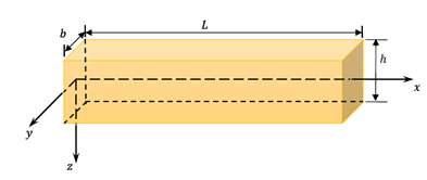
Figure 1 Schematic diagram for the nanobeam.

For a one–dimensional problem, the differential form of the constitutive Eq. (9) after using Eqs. (1) and (14) can be expressed as:^32,33

${\sigma }_x-\xi \frac{{\partial }^2{\sigma }_x}{\partial x^2}=-E_{0}F\left(T_0\right)\left[\frac{{\partial }^{2}w}{\partial x^2}+{\alpha }_T\theta \right]$ (15)

$\frac{{\partial }^{2}M}{\partial x^2}=\rho A\frac{{\partial }^{2}w}{\partial t^2}$ (16)

With aid of Eq. (15), the flexure moment is given by

$M\left(x,t\right)-\xi \frac{{\partial }^{2}M}{\partial x^2}=-I{E}_{0}F\left(T_0\right)\left[\frac{{\partial }^{2}w}{\partial x^2}+{\alpha }_T{M}_T\right]$ (17)

$M_T=\frac{12}{h^3}{\int }_{-h/2}^{h/2}\theta \left(x,z,t\right)zdz$ (18)

$\frac{{\partial }^{4}w}{\partial x^4}+\frac{\rho }{I{E}_{0}F\left(T_0\right)}\left(\frac{{\partial }^{2}w}{\partial t^2}-\xi \frac{{\partial }^{4}w}{\partial t^2\partial x^2}\right)+{\alpha }_t\frac{{\partial }^2{M}_T}{\partial x^2}=0$ (19)

$M\left(x,t\right)=\xi A\rho \frac{{\partial }^{2}w}{\partial t^2}-I{E}_{0}F\left(T_0\right)\left[\frac{{\partial }^{2}w}{\partial x^2}+{\alpha }_t{M}_T\right]$  (20)

There is no heat flow across the upper and lower surfaces of the nanobeam (thermally insulated), so that$\frac{\partial \theta }{\partial z}$  should be vanish at the upper and lower surfaces of the nanobeam$z=\pm h/2$ . For a very nanobeam, assuming that the increment temperature varies in a sinusoidal form along the thickness direction. That is

$\theta \left(x,z,t\right)=\Theta \left(x,t\right)\sin \left(\frac{\pi z}{h}\right)$ (22)

Substituting Eq. (22) into Eq. (19), one can get the motion equation of the nanobeams as

$\frac{{\partial }^{4}w}{\partial x^4}+\frac{\rho A}{E_{0}F\left(T_0\right)}\left(\frac{{\partial }^{2}w}{\partial t^2}-\xi \frac{{\partial }^{4}w}{\partial t^2\partial x^2}\right)+\frac{24{\alpha }_t}{h{\pi }^2}\frac{{\partial }^2\Theta }{\partial x^2}=0$ (23)

Also, the flexure moment can be determined from Eqs. (20) and (22) as $M\left(x,t\right)=\xi A\rho \frac{{\partial }^{2}w}{\partial t^2}-I{E}_{0}F\left(T_0\right)\left[\frac{{\partial }^{2}w}{\partial x^2}+\frac{24{\alpha }_t}{h{\pi }^2}\Theta \right]$ (24)

$\frac{{\partial }^2\Theta }{\partial x^2}-\frac{{\pi }^2}{h^2}\frac{{\partial }^2\Theta }{\partial z^2}=\left(\text{δ}+\frac{{\tau }_0^{\alpha }}{\alpha !}\frac{{\partial }^{\alpha }}{\partial t^{\alpha }}\right)\left[\frac{1}{k}\frac{\partial \Theta }{\partial t}-\frac{{\gamma }_0{T}_0{\pi }^{2}h}{24K_0}\frac{\partial }{\partial t}\left(\frac{{\partial }^{2}w}{\partial x^2}\right)\right]$  (25)

$\begin{array}{l}\left\{x^{\prime },z^{\prime },u^{\prime },w^{\prime },L^{\prime },h^{\prime }\right\}=c_0{\eta }_0\left\{x,z,u,w,L,h\right\}, \left\{t^{\prime },\tau {\text{'}}_0,{\xi }^{\prime }\right\}=c_0^2{\eta }_0\left\{t,{\tau }_0,{\eta }_0\xi \right\},\\ {\Theta }^{\prime }=\frac{\Theta }{T_0}, {{\sigma }^{\prime }}_x=\frac{{\sigma }_x}{E_0}, M^{\prime }=\frac{M}{c_0{\eta }_{0}I{E}_{0}F\left(T_0\right)}, c_0=\sqrt{\frac{E_0}{\rho }}.\end{array}$ (26)

So, the basic equations in nondimensional forms are simplified as (dropping the primes for convenience)

$\begin{array}{l}\frac{{\partial }^{4}w}{\partial x^4}+A_1\left(\frac{{\partial }^{2}w}{\partial t^2}-\xi \frac{{\partial }^{4}w}{\partial t^2\partial x^2}\right)=-A_2\frac{{\partial }^2\Theta }{\partial x^2}\\ \left(\frac{{\partial }^2}{\partial x^2}-A_4\right)\Theta =\left(1+\frac{{\tau }_0^{\alpha }}{\alpha !}\frac{{\partial }^{\alpha }}{\partial t^{\alpha }}\right)\left[\frac{\partial \Theta }{\partial t}-A_5\frac{\partial }{\partial t}\left(\frac{{\partial }^{2}w}{\partial x^2}\right)\right]\end{array}$ (27)

$M\left(x,t\right)=A_1\left(\xi \frac{{\partial }^{2}w}{\partial t^2}-\frac{{\partial }^{2}w}{\partial x^2}\right)-A_2\Theta$ (28)

$A_1=\frac{12}{F\left(T_0\right)h^2},A_2=\frac{24T_0{\alpha }_t}{{\pi }^{2}h}, A_3= \xi A_1,A_4=\frac{{\pi }^2}{h^2},A_5=\frac{{\gamma }_0\text{k}{\pi }^{2}h}{24K_0}$

To solve the problem, the initial and boundary conditions must be taken into consideration. The homogeneous initial conditions are taken as

$\Theta \left(x,0\right)=\frac{\partial \Theta \left(x,0\right)}{\partial t}=0=\text{w}\left(x,0\right)=\frac{\partial \text{w}\left(x,0\right)}{\partial t}$ (29)

$\text{w}\left(0,\text{t}\right)=\text{w}\left(L,\text{t}\right)=0=\frac{{\partial }^2\text{w}\left(0,\text{t}\right)}{\partial x^2}=\frac{{\partial }^2\text{w}\left(L,\text{t}\right)}{\partial x^2}$  (30)

$\Theta \left(x,t\right)={\Theta }_0\{\begin{array}{c}0, t\le 0,\\ \frac{t}{t_0}, 0\le t\le t_0\\ 1, t>0\end{array},$ (31)

$\frac{\partial \Theta }{\partial x}=0 \text{on} x=L$ (32)

The closed form solution of the governing and constitutive equations can be possible by adapting the Laplace transformation method. Taking the Laplace transform defined by the relation

$\overline{f}\left(x,t\right)={\int }_0^{\infty }f\left(x,t\right)e^{-st}dt$ (33)

$\begin{array}{l}\left(\frac{d^4}{d{x}^4}-A_3{s}^2\frac{d^2}{d{x}^2}+A_1{s}^2\right)\overline{w}=-A_2\frac{d^2\overline{\Theta }}{d{x}^2}, \\ \left(\frac{{\partial }^2}{\partial x^2}-B_1\right)\overline{\Theta }=-B_2\frac{{\partial }^2\overline{w}}{\partial x^2},\end{array}$ (34)            

$\overline{M}\left(x,t\right)=A_1\left(\xi s^2\overline{w}-\frac{d^2\overline{w}}{d{x}^2}\right)-A_2\overline{\Theta }$ (35)

$\left(D^6-A{D}^4+B{D}^2-C\right)\left\{\overline{\Theta },\overline{w}\right\}\left(x\right)=0,$ (36)

$A=A_3{s}^2+A_2{B}_2+B_1, B=A_1{s}^2+B_1{A}_3{s}^2, C=A_1{B}_1{s}^2,D=\frac{d}{dx}$ (37)

$m^6-A{m}^4+B{m}^2-C=0,$ (39)

${\beta }_n=-\frac{m_n^2{B}_2}{m_n^2-B_1}$ (41)

The axial displacement after using Eq. (40) takes the form $\overline{u}\left(x\right)=-z\frac{d\overline{w}}{dx}=z{\displaystyle \sum }_{n=1}^3{m}_n\left(C_n{\text{e}}^{-m_{n}x}-C_{n+3}{\text{e}}^{m_{n}x}\right).$ (42)

Substituting the expressions of $\overline{w}$ and $\overline{\Theta }$ from (40) into (36), we get at the solution for the bending moment $\overline{M}$ as follows:

$\overline{M}\left(x\right)={\displaystyle \sum }_{n=1}^3\left(A_3{s}^2-m_n^2-A_2{\beta }_n\right)\left(C_n{\text{e}}^{-m_{n}x}{C}_{n+3}{\text{e}}^{m_{n}x}\right).$ (43)

In addition, the strain will be

$\overline{e}\left(x\right)=\frac{d\overline{u}}{dx}=-z{\displaystyle \sum }_{n=1}^3{m}_n^2\left(C_n{\text{e}}^{-m_{n}x}+C_{n+1}{\text{e}}^{m_{n}x}\right).$ (44)

$\begin{array}{l}\overline{w}\left(0,s\right)=\overline{w}\left(L,s\right)=0, \\ \frac{{\partial }^2\overline{w}\left(0,s\right)}{\partial x^2}=\frac{{\partial }^2\overline{w}\left(L,s\right)}{\partial x^2}=0,\\ \frac{\partial \overline{\Theta }\left(0,s\right)}{\partial x}={\Theta }_0\left(\frac{1-e^{-s{t}_0}}{s^2{t}_0}\right)=\overline{G}\left(s\right), \\ \frac{\partial \overline{\Theta }\left(L,s\right)}{\partial x}=0 \end{array}$ (45)

$\begin{array}{l}{\displaystyle \sum }_{n=1}^3\left(C_n+C_{n+1}\right)=0,\\ {\displaystyle \sum }_{n=1}^3\left(C_n{\text{e}}^{-m_{n}L}+C_{n+1}{\text{e}}^{m_{n}L}\right)=0, \end{array}$  (46)

$\begin{array}{l}{\displaystyle \sum }_{n=1}^3{m}_n^2\left(C_n+C_{n+1}\right)=0,\\ {\displaystyle \sum }_{n=1}^3{m}_n^2\left(C_n{\text{e}}^{-m_{n}L}+C_{n+1}{\text{e}}^{m_{n}L}\right)=0, \end{array}$  (47)

$\begin{array}{l}{\displaystyle \sum }_{n=1}^3{m}_n\left({\beta }_n{C}_n-{\beta }_{n+1}{C}_{n+1}\right)=-\text{G}\left(\text{s}\right),\\ {\displaystyle \sum }_{n=1}^3{m}_n\left({\beta }_n{C}_n{\text{e}}^{-m_{n}L}-{\beta }_{n+1}{C}_{n+1}{\text{e}}^{m_{n}L}\right)=0, \end{array}$  (48)

The solution of the above system of linear equations gives the unknown parameters,. In order to determine the studied fields in the physiacl domain, the Riemann-sum approximation method is used to obtain the numerical results. The details of these methods can be found in Honig & Hirdes.33

Special case

The following special cases can be obtained from the system of Eqs. (1), (8) and (9):

1. The equations of a coupled theory of nonlocal thermoelasticity with temperature-dependent mechanical properties result from (1), (8), in the limiting caseand (11) by lettingand putting.
2. The equations of a coupled theory of local thermoelasticity with temperature-dependent mechanical properties result from (1), (8), in the limiting caseand (11) by lettingand putting.
3. The equations of a coupled theory of nonlocal thermoelasticity with temperature-independent mechanical properties result from (1), (8) and (9), in the limiting caseand (11) by letting,and putting.
4. The equations of a coupled theory of local thermoelasticity with temperature-independent mechanical properties result from (1), (8) and (9), in the limiting caseby lettingand putting.
5. The equations of a generalized theory of nonlocal thermoelasticity with temperature-dependent mechanical properties without fractional derivatives are obtained from Eqs. (1), (8) and (9) by letting the fractional parameterand putting.
6. The equations of a generalized theory of nonlocal thermoelasticity with temperature-independent mechanical properties without fractional derivatives are obtained from Eqs. (1), (8) and (9) by letting the fractional parameterand puttingand.
7. The equations of the generalized nonlocal thermoelasticity without energy dissipation with temperature-dependent mechanical properties without fractional derivatives result from Eqs. (1), (8) and (9) by letting,and.

In the present work, the thermoelastic coupling effect is analyzed by considering a beam made of silicon (Table 1).

Also, the length−to−thickness ratio of the nanobeam is fixed asand the dimensional parameters carried out in the numerical simulations areand. For all numerical calculations Mathematica programming Language has been used. The numerical calculations of the flexure momentthermodynamical temperature, displacement, lateral vibrationand strainhave been considered for various values of the nonlocal parameterfractional orderthickness of nanobeam and periodic frequency. The results are investigated graphically in Figures 2−17 in the wide range ofat different positions of. Some plots consider the present quantitis throug the length of the beam and others take into account both the length and thickness directions.

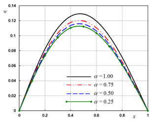
Figure 2 The transverse deflection with different fractional order parameter .

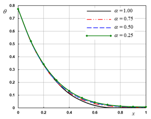
Figure 3 The temperature with different fractional order parameter .

Figure 4 The displacement with different fractional order parameter .

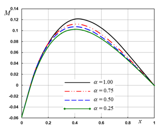
Figure 5 The flexure moment with different fractional order parameter .

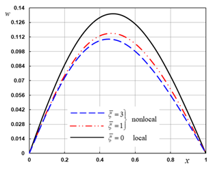
Figure 6 The transverse deflection with different nonlocal parameter .

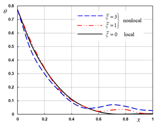
Figure 7 The temperature with different nonlocal parameter .

Figure 8 The displacement with different nonlocal parameter .

Figure 9 The flexure moment with different nonlocal parameter .

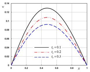
Figure 10 The transverse deflection with different ramping time .

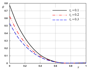
Figure 11 The temperature with different ramping time .

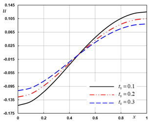
Figure 12 The displacement with different ramping time .

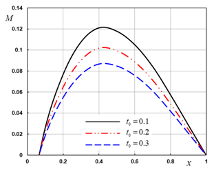
Figure 13 The flexure moment with different ramping time .

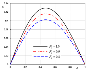
Figure 14 The transverse deflection in the case of temperature−independent properties.

Figure 15 The temperature in the case of temperature−independent properties.

Figure 16 The displacement in the case of temperature−independent properties.

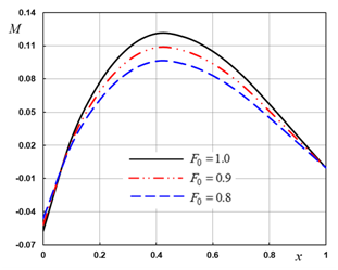
Figure 17 The flexure moment in the case of temperature−independent properties.

From the results we obtained it is clear that, the field quantities such as the deflection, temperature, displacement, and bending moment distributions depend not only on the timeand space coordinate, but also depend on the fractional parameter, nonlocal parameter ramping time parameterand effect of reference temperature. Numerical calculations and graphs have been divided into four cases. In this work, the obtained results have been compared with the results obtained previously in.^22,23,35,4

The effect of the fractional order parameter

In the first case, we represent the dimensionless lateral vibration, thermodynamic temperature, displacement, and bending moment at different fractional order parameter  to stand on the effect of this parameter on all the studied fields (Figures 2−5). The computations were carried out for wide range of , for different values of the parameter  with wide rangewhen,, and.The different values of the parameter,describes two types of conductivity (weak conductivity,,normal conductivity,), respectively. From the different figures it is observed that the nature of variations of all the field variables for fractional order parameter is significantly different. The difference is more prominent for higher values of fractional derivative. This observation is consistent with previous results in.²²We also observes the following important facts from Figures 3−6.

1. The lateral vibrationdistribution has large change against to fractional order parameter. Also, the lateral vibration increases with the increase of the parameter.
2. From figure 1, lateral vibration atis zero as shown, which agrees with the boundary condition prescribed. This coincided with the mechanical boundary condition that the two ends of the nanobeam are clamped.
3. We observed that at the lateral vibrationreaches a maximum value at some distance from the surface of the nanobeam and then it decreases with the increase of distance.
4. The temperature distribution have small differences for different values of.
5. Figure 3 indicate that thetemperature has a maximum value at boundaryand decreases smoothly and finally tends to zero after some distance (which satisfy the boundary conditions).
6. Figure 3 shows that the displacementincreases as It can be observed that the fractional order parameterhas a great effects on the displacement distribution.
7. From Figure 4 it is observed that the bending momentincreases as the distanceincreases and then it decreases with the increase of distance. Figure 5 shows that the bending moment larg dependent on the variation of the fractional order parameter.
8. According to these results, we have to construct a new classification to all the materials according to its fractional parameter, where this parameter becomes new indicator of its ability to conduct the thermal energy; confirms the results obtained in.²²

The effect of the nonlocal parameter

Figures 6−9 describe the temperature, displacement, lateral vibration and bending moment field distributions for different values of nonlocal parameter. In this case, we notice that when the nonlocal parametervanishingindicates the old situation (local model of elasticity) while other values indicate the nonlocal theories of elasticity and thermo elasticity. The figures 6−9 show that this parameter has significant effect on all the fields. The waves reach the steady state depending on the value of the nonlocal parameter. The conclusion remarks from the Figures can be shortened as follows:

1. The lateral vibrationdecrease when the value of increases while the values of the bending momentincreases when the value of
2. It can be seen from Figure 7 that the temperaturesmall dependent on the variation of nonlocal parameter .
3. From Figure 5, the values of the displacementstart increasing with the nonlocal parameter in the range,thereafter increasing to maximum amplitudes in the range. This shows the difference between the local generalized thermoelasticity and the nonlocal generalized thermoelasticity models.
4. It can be seen from Figure 9 that the bending moment larg dependent on the variation of nonlocal parameter.
5. As in,^23,35,40 the field variables have pronounced sensitive to the variation of the nonlocal parameter.

The effect of the ramping time parameter

This case illustrating how the field quantities vary with the different values of the ramping time parameterwith constant,, and. The numerical results are obtained and presented graphically in Figures 10−13. We can see the significant effect of the ramping time parameteron all the studied fields. Also, we can conclude that:

1. The increasing in the value of the ramping time parameter causes decreasing in the values of thelateral vibration, temperatureand bending momentwhich is very obvious in the peek points of the curves.
2. Also, the values of the displacementstart decreasing with the ramping time parameter in the range, thereafter increasing to maximum amplitudes in the range.
3. It can be observed that the ramping time parameterhas great effects on the distribution of field quantities. This is also consistent with what has been obtained in.⁴⁰

The effect of the temperature−independent modulus

This case presents the effect of temperature−dependent properties (reference temperature) on the field variables for fixed values of the ramping time parameterand the nonlocal parameteraccording to the equation. For a comparison of the results, the lateral vibration, the temperature, the displacement, and the bending moment of the nano−beam are shown in Figures 14−17. We found that, the increasing in the value of causes increasing in the values of the lateral vibration, temperature, displacement fields which is very obvious in the peek points of the curves. When the modulus of elasticity is a linear function of reference temperatureand in the case of a temperature−independent modulu. On the other hand, high sensitivity is observed for the effect of the reference temperature on all of the studied variables. This also agrees with what Zenkour has reached in.⁴⁰

The thermal and mechanical properties of materials vary with temperature, so that the temperature dependent on material properties must be taken into consideration in the thermal stress analysis of these elements. In this work, a new model of nonlocal generalized thermoelasticity based upon Euler–Bernoulli theory for nanobeams is constructed. The vibration characteristics of the deflection, temperature, displacement and bending moment of nanobeam subjected to ramp–type heating are investigated. The effects of the nonlocal parameter, fractional order parameterand the ramping time parameteron the field variables are investigated. Numerical technique based on the Laplace transformation has been used. The effects of the nonlocal parameter, reference temperature and the ramping time parameter on all the studied field quantities have been shown and presented graphically.

According to the results shown in all figures, it is find that:

1. The nonlocal parameterhas significant effects on all the studied fields.
2. The effect of the fractional parameter on all the studied fields is very significant.
3. The thermo elastic stresses, displacement and temperature have a strong dependency on the ramping time parameter.
4. The parameterand the dimension cause significant changes on all the studied fields and the phenomenon of finite speeds of propagation are manifested in all figures.
5. New classification of the materials must be constructed according to the fractional parameter which describes the ability of the material to conduct the heat.
6. This study is very important for micro scale problems because in these cases the material parameters are temperature dependent.

None

The author declares that there is no conflict of interest.

1. Caputo M. Linear model of dissipation whose Q is almost frequency independent−II. Geophysics Journal of the Royal Astronomical Society. 1967;13(5):529–539.
2. Caputo M, Mainardi F. A new dissipation model based on memory mechanism. Pure and Applied Geophysics. 1971;91(1):134–147.
3. Povstenko YZ. Fractional heat conduction equation and associated thermal stress. J Therm Stress. 2005;28(1);83–102.
4. Povstenko YZ, Thermoelasticity that uses fractional heat conduction equation. J Math Sci. 2009;162(2):296–305.
5. Jiang X, Xu M. The time fractional heat conduction equation in the general orthogonal curvilinear coordinate and the cylindrical coordinate systems. Physica A. 2010;389(17):3368–3374.
6. Stefan G Samko, Anatolij A Kilbas, Oleg I Marichev. Fractional Integrals and Derivatives, Theory and Applications. Gordon and Breach, Amsterdam. 1993.
7. Gorenflo R, Mainardi F. Fractional calculus: Integral and differential equations of fractional order. Fractals and Fractional Calculus in Continuum Mechanics. 1997;223–276.
8. Mainardi F. Applications of fractional calculus in mechanics. In: Rusev P, Dimovski I, Kiryakova V (Eds.): Transform Methods and Special Functions. Bulgarian Academy of Sciences, Sofia. 1998:309–334.
9. Lord HW, Shulman Y. A generalized dynamical theory of thermoelasticity. J Mech Phys Solids. 1967;15(5):299–309.
10. Green AE, Lindsay KA. Thermoelasticity. Journal of Elasticity. 1972;2(1):1–7.
11. Green AE, Naghdi PM. Thermoelasticity without energy dissipation. Journal of Elasticity. 1993;31(3):189–208.
12. Sherief HH, El−Sayed AMA, Abd El−Latief AM. Fractional order theory of thermoelasticity. Int J Solids Struct. 2010;47(2): 269–275.
13. Ezzat MA. Magneto−thermoelasticity with thermoelectric properties and fractional derivative heat transfer. Physica B. 2011;406(1):30–35.
14. Jumarie G. Derivation and solutions of some fractional Black−Scholes equations in coarse−grained space and time. Application to Merton's optimal portfolio. Computers & Mathematics with Applications. 2010;59(3):1142–1164.
15. El-Karamany S and Ezzat MA. Convolutional variational principle, reciprocal and uniqueness theorems in linear fractional two−temperature thermoelasticity. J of Thermal Stresses. 2011;34(3):264–284.
16. Noda N. Thermal stresses in materials with temperature–dependent properties, thermal stresses I, Richard B. Hetnarski (Editor), North–Holland, Amsterdam. 1986.
17. Hasselman DPH, Heller RA. Thermal stresses in sever environments. Plenum Press: New York; 1980.
18. Tanigawa Y. Some Basic Thermoelastic Problems for Non– homogeneous Structural Materials. Appl Mech Rev. 1995;48(6):287–300.
19. Magdy A Ezzat, El-Karamany AS, Alla A El–Bary. Magneto–thermoelasticity with two fractional order heat transfer. Journal of the Association of Arab Universities for Basic and Applied Sciences. 2016;19:70–79.
20. Abouelregal AE, Zenkour AM. Effect of fractional thermoelasticity on a twodimensional problem of a mode I crack in a rotating fibre–reinforced thermoelastic medium. Chinese Physics B. 2013;22(10):108102.
21. Zenkour AM, Abouelregal AE. State–space approach for an infinite medium with a spherical cavity based upon two–temperature generalized thermoelasticity theory and fractional heat conduction. Zeitschrift fur angewandte Mathematik und Physik. 2014;65(1):149–164.
22. Mashat DS, Zenkour AM, Abouelregal AE. Fractional order thermoelasticity theory for a half-space subjected to an axisymmetric heat distribution. Mechanics of Advanced Materials and Structures. 2015;22(11):925–932.
23. Zenkour AM, Abouelregal AE. The Nonlocal Dual Phase Lag Model of a Thermoelastic Nanobeam Subjected to a Sinusoidal Pulse Heating. International Journal for Computational Methods in Engineering Science and Mechanics. 2015;16(1):44–52.
24. Ahmed E Abouelregal. Fibre–Reinforced Generalized Anisotropic Thick Plate with Initial Stress under the Influence of Fractional Thermoelasticity Theory. Advances in Applied Mathematics and Mechanics. 2017;9(3):722–741.
25. Fang DN, Sun YX, Soh AK. Analysis of frequency spectrum of laser–induced vibration of microbeam resonators. Chinese Phys Lett. 2006;23(6):1554–1557.
26. Kidawa–Kukla J. Application of the Green functions to the problem of the thermally induced vibration of a beam. J Sound Vib. 2003;262(4):865–876.
27. Manolis GD, Beskos DE. Thermally induced vibrations of beam structures. Comput Meth Appl Mech Eng. 1980;21(3):337–355.
28. Eringen AC, Edelen DGB. On nonlocal elasticity. Int J Eng Sci. 1972;10(3):233–248.
29. Eringen AC. On differential equations of nonlocal elasticity and solutions of screw dislocation and surface waves. J Appl Phys. 1983;54(9):4703–4710.
30. Peddieson J, Buchanan R, McNitt RP. Application of nonlocal continuum models to nanotechnology. Int J Eng Sci. 2003;41(3):305–312.
31. Lu P, Lee HP, Lu C, et al. Application of nonlocal beam models for carbon nanotubes. Int J Solids Struct. 2007;44(16):5289–5300.
32. Eringen AC. Nonlocal continuum field theories. Springer. New York;2002.
33. Zenkour AM, Abouelregal AE, Alnefaie KA, et al. A refined nonlocal thermoelasticity theory for the vibration of nanobeams induced by ramp–type heating. Applied Mathematics and Computation. 2014;248:169–183.
34. Zenkour AM, Abouelregal AE. Vibration of FG nanobeams induced by sinusoidal pulse heating via a nonlocal thermoelastic model. Acta Mechanica. 2014;225(12):3409–3421.
35. Zenkour AM, Abouelregal AE. Nonlocal thermoelastic nanobeam subjected to a sinusoidal pulse heating and temperature−dependent physical properties. Microsystem Technologies. 2015;21(8):1767–1776.
36. Miller KS, Ross B. An introduction to the fractional integrals and derivatives. Theory and applications. John Wiley and Sons Inc: New York; 1993.
37. Podlubny. Fractional differential equations. Academic press: New York; 1999.
38. Lomarkin VA. The Theory of Elasticity of Non–homogeneous Bodies. Moscow; 1976.
39. Szuecs F, Werner M, Sussmann RS, et al. Temperature dependence of Young's modulus and degradation of chemical vapor deposited diamond. J Appl Phys. 1999;86:6010–6017.
40. Zenkour AM. Effect of temperature–dependent physical properties on nanobeam structures induced by ramp–type heating. KSCE J Civ Eng. 2017;21(5):1820–1828.
41. Tzou D. Macro–to–Micro Heat Transfer. Taylor & Francis: Washington DC; 1996.