In this paper, we examine dynamic changes in cardiac inter-beat intervals to explore these differences in cardiac control. Moment-to moment changes in RR intervals during premeditation state were compared with the corresponding values during meditation state. For each state, every RR interval was plotted against the previous interval (Poincaré plot) and each change in the inter-beat interval was plotted against the previous change (sequence trend analysis or quadrant analysis plot). The variability in inter-beat intervals is an indicator of the dynamic interaction and the balance between the sympathetic and parasympathetic branches of the autonomic nervous system (ANS). The sympathetic branch decreases the inter-beat intervals, while the parasympathetic branch increases the inter-beat intervals. In this study we evaluated the ANS during two concentration meditation techniques (Kundalini yoga and Chi meditations) using the above two nonlinear methods, namely, Poincaré plot and sequence trend analyses. It is found through both the methods that the complex dynamics of the RR interval series is lowered during meditation. Further, during premeditation state there is parasympathetic dominance while during meditation state there is sympathetic dominance, irrespective of the type of meditation. Kundalini yoga group meditators showed higher differences than Chi group meditators.

Keywords: autonomic nervous system, heart rate variability, meditation, poincaré plot, rr interval, sequential trend analysis

Found in cultures, spiritual traditions, and healing practices throughout the world, meditation is a mind-body practice with different approaches and variations, which began probably more than five thousand years ago. Since then it has developed and practiced to understand consciousness and improve health conditions. All these meditation techniques can be broadly classified under two categories: concentration meditation and insight meditation.¹ In the former, attention is focused on the breath to still the mind. As the meditator concentrates on the breath, the mind gets absorbed in the inhalation and exhalation which may lead a state of silence mind, usually called The Samadhi state. The insight meditation involves opening the attention to become aware of the continuously passing of sensation and the feeling without getting involved into the thoughts about them.² Meditation is a complex physiological process which affects psychological, behavioral, neural and autonomic functions and is regarded as an altered state of consciousness, different from wakefulness, relaxation at rest and sleep.³⁻⁵ Many have shown that the meditation practice leads to functional changes in physiological states of humans.⁶⁻⁸ It is found that most of the meditation techniques affect the ANS which in turn regulates organs and muscles thereby controlling vital functions such as heart beat, respiration, and digestion. In fact respiration is one of the autonomic functions that can be controlled and affect the functioning of the ANS.⁹ As an implication many of the meditation practices consider respiration, mind and body as linked, with respiration having a central role.

HRV analysis is fast emerging as a noninvasive research and clinical tool for assessing cardiac and ANS function.^10,11 The analysis of HRV, in general, is a difficult task due to the nonlinearity and nonstationarity of the RR interval time series. Traditional HRV analysis methods are based on linear methods in the time, frequency or time-frequency domains. Such methods have been widely used to study sympathetic and parasympathetic activities. These methods assume stationarity of the time-series within the sample, an assumption that is often violated in the heart rate series. Heart rate often changes in an asymmetric fashion and this leads to complexity in the interpretations of the results. Nonlinear methods are being explored since it has been found that nonlinear phenomena are involved in the genesis of HRV.¹²⁻¹⁴ Many studies have shown that HRV is reduced in various diseases and old age.^15,16 Even in predicting mortality of survivors of myocardial infarction, reduced HRV is used as a marker.^17,18 In the context of meditation, the study of HRV offers a unique approach to view into the complex mind-body connection that exists behind the regulation of life processes, such as blood circulation, and breathing. Analysis of HRV signals is important when studying the ANS because it helps in evaluating the dynamic interaction and the equilibrium between the sympathetic and parasympathetic influences on the heart rate. The sympathetic branch of nervous system increases the heart rate, resulting in shorter beat intervals. On the other hand, the parasympathetic branch decreases the heart rate, resulting in longer beat intervals. Thus the HRV can be evaluated based on beat intervals or RR intervals. Meditation, perhaps, is well suited to investigate intrinsic properties of the ANS since it involves a state of complete physical immobility and almost absence of voluntary efforts. Poincaré plot has been used by Goshvarpour et al.¹⁹ as visual tool just to show that the trajectories in the plot spread out during meditation compared to premeditation. But no quantitative analysis of the Poincaré plot has been made.¹⁹ Poincaré plot of the generalized angle map was used by Anilesh Dey et al.²⁰ to distinguish premeditation and meditation states. The length of the major axis was found to increase in the meditation state compared to premeditation state and hence the two states to have different physiology.²⁰ Goswami et al.²¹ used second-order difference plot to visually differentiate meditative state from normal physiological state. They found that in the state of meditation the rates of HRVs correlate with each other and the external stimuli do not affect the physiological conditions. The situation was reversed during the non-meditative state where external stimuli affected the physiological conditions. As an implication they concluded that the meditative states have a completely different physiology from the non-meditative states.²¹ ANS during meditation has been evaluated by different methods^2,22−26 but not with Poincaré plot and sequence trend analyses. Both these nonlinear methods permit assessment of autonomic balance, besides measuring different aspects of HRV. Poincaré plot width can be used as a specific measure of parasympathetic activity. Sequence trend analysis permits the nature of cardiac interval sequencing and permits the evaluation of both sympathetic and parasympathetic activities. In this study we analyze the HRV during two specific meditative techniques based on concentration meditation:

1. Chinese Chi and
2. Kundalini yoga by means of two nonlinear dynamics methods: Poincaré plot analysis and sequence trend analysis. An important advantage of both of these methods is that they are independent of the stationarity of the RR interval time series.²⁷

ECG records

The RR interval time series used in this study were during two specific meditative techniques based on concentration meditation:

1. Chi meditation and
2. Kundalini yoga meditation, all from the benchmark PhysioNet database.²⁸

The Chi meditators were relative novices in their practice of Chi meditation. However, the Kundalini yoga meditators were considered to be at an advance stage of meditation training. The chi meditation group included 8 subjects, 5 women and 3 men (age range 26-35, with mean = 29 years). The Holter monitor recording was made for 10 hours during which the subjects went through their daily activities. At approximately 10 hours into the recording they each practiced one hour of meditation. The beginning and ending times of meditation were delineated with event marks. During the meditation sessions the Chi meditators sat quietly, listening to the taped guidance of the Master. They were instructed to breathe spontaneously while visualizing the opening and closing of a perfect lotus in the stomach. The Kundalini yoga meditation group included 4 subjects, 2 women and 2 men (age range 20-52, with mean = 33 years). The Holter monitor recording was made for one and half hours. 15 minutes of baseline quiet breathing were recorded before the 1 hour of meditation. The meditation protocol consisted of a sequence of breathing and chanting exercises, performed while seated in a cross-legged posture. The beginning and ending times of the various meditation sub-phases were delineated with event marks. All the pre-meditation and meditation RR interval records are passed through a square filter to eliminate artifacts, premature beats and outliers, if any, and then filtered using an 8-point moving average filter to remove high-frequency noise like interspersions and muscle noise. Each record in the Chi and Kundalini yoga groups then was normalized.

Poincaré plot analysis

Poincaré plot is a geometrical representation of a time series into a Cartesian plane, where the values of each pair of successive elements of the time series define a point in the scatter plot.²⁹ In the case of HRV analysis each RR interval is plotted against its predecessor in the scatter plot. This procedure provides an indication of the probability of occurrence of one interval from its predecessor and allows assessment of short-term dynamic properties of RR interval variation. Each plots shows

1. Beat-to-beat variability (variation in RR_n for a given value of RR_n-1), which is reflected in the scatter of values on the y-axis for a given value on the x-axis and
2. Overall variation, which is reflected in absolute extent of dispersion of dispersion of points along the axes.

A conventional Poincaré plot is analyzed quantitatively by evaluating SD2 and SD1, the dispersions of points along the line y=x and the line y=-x+2*RR_m, respectively, where RR_m represents the mean of the RR interval series. The intersection of these two lines is given by (RR_m, RR_m). The scatter plot width (SD1) is closely related to short-term variability in RR intervals; scatter plot length (SD2) is correlated with long-term variability in RR intervals. Further, a strong correlation has been established between SD1 and high frequency power of HRV (modulated by parasympathetic nervous system) and a similar correlation between SD2 and both low and high frequency power of HRV (modulated by parasympathetic and sympathetic nervous system). A reduced value of SD1 implies decreased parasympathetic activity and vice versa. Similarly, reduced value of SD2 implies decreased sympathetic activity and vice versa. The ratio SD2/SD1 serves as an approximate indicator of sympathovagal balance.³⁰ Higher values of this ratio indicate an increased sympathetic activity and/or decreased parasympathetic activity. Further, the descriptor S=π SD1 SD2, which corresponds to the area of the imaginary ellipse on the Poincaré plot, serves an indicator of total HR variability. Larger values of S imply higher variability and vice versa. The dispersion of the points (variability) in the Poincaré plot is related to complex dynamics of the time series. An increased temporal dispersion indicates more complex dynamics.

Sequence trend analysis

Sequence trend analysis, sometimes called, quadrant analysis, is a novel nonlinear approach where the sequencing of cardiac accelerations and decelerations is revealed after the strong correlation between adjacent RR intervals is removed in both the time domain and scatter plot analyses.²⁷ This permits time dependent dynamics of HRV to be assessed. Here we produce scatter plots of first differences of the data which graph x(n+2)–x(n+1) verses x(n+1)–x(n), where x(n) is the value of the RR interval time series at time n. These second order plots centered about the origin, facilitate graphical visualization of the degree of variability in the time series. These plots reveal the serial dependencies of cardiac accelerations and decelerations. The scatter plot of first differences of the data consists of values distributed on an area around the origin in four quadrants as shown in Fig. 1. Each quadrant represents the direction and the extent of change in RR interval length from one interval to the next. Four patterns can be identified: +/+ (quadrant 1; a lengthening-sequence, cardiac deceleration), +/- or -/+ (quadrant 2/4 respectively; balanced sequences), and finally -/- (quadrant 3; a shortening-sequence, cardiac acceleration). Events of each type are counted by quadrant. These plots, which show dependencies of changes in interval lengths from previous changes, contain additional information on short-term heart rate dynamics. Since each quadrant indicates direction of two consecutive changes in the interval length, the scatter plots of first differences of the time series demonstrate 1) the ratio of short-to-long term changes in the heart rate and 2) the trends of variation in the heart rate.³¹

Ratio of high frequency to low frequency heart rate variation

The high frequency heart rate variation is characterized by rapid changes in the slope of the RR interval time series (an increase in the RR interval length followed by a decrease and vice versa) in the time domain.³² Thus high-frequency variation is reflected by points in quadrants 2 and 4 of Figure 1. Low-frequency heart rate variation, on the other hand, is characterized by many sequential increases in interval length or many sequential decreases in interval length. The low-frequency variation is reflected by points in quadrants 1 and 3.³²

Figure 1 Scatter plot of first difference of RR intervals (Quadrant occupancy histogram).

Trends of variation in heart rate

If variation from one RR interval to the next occurred randomly and independently, then all the four quadrants would be expected to have an almost equal distribution of points. If, on the other hand, the heart rate tended to decrease rapidly (increasing in the interval lengths) and increase more slowly (decreasing in the interval lengths), there would be a greater number of intervals representing increasing heart rates (decreasing RR intervals).³² As a consequence more number of points will fall in the quadrants 3 and 4 than in 1 and 2. The opposite is true, if the heart rate tended to increase rapidly (decreasing in the interval lengths) and decrease more slowly (increasing in the interval lengths).³² The scatter plot of first differences of the data, which graphs x(n+2)–x(n+1) verses x(n+1) – x(n), is quantified by the total number of points in each quadrant. Every quadrant represents one type of event / pattern.

Central tendency measure (CTM)

Scatter plot of first differences are useful in modeling biological systems, such as hemodynamic and HRV, represent the degree of theoretical chaos.³³ In this approach, instead of identifying the time series as chaotic or non-chaotic, the degree of variability or chaos is evaluated. Cohen et al.³⁴ have proposed a central tendency measure which quantifies the degree of variability in a scatter plot of the first difference of the series.³⁴ Given a circular region of radius r, about the origin, the CTM is measured as the ratio of the number of points (in all the four quadrants together) that fall within this radius r, to the total number of points in the entire plot. This count involves the number of successive rates that include all sign combinations or quadrant regions within radius r. If N is the total number of points in the time series the scatter plot will have N–2 points. CTM is defined, by selecting a circular region of radius r about the origin in the scatter plot and counting the number of points (in all the four quadrants together) that fall within this region and dividing it by the total number of points, as below.

$CTM\left(r\right)={\sum }_i\delta \left(d_i\right)/\left(N-2\right)1\le i\le N-2$ (1)

where,$\delta \left(d_i\right)=1,if{\left[X^2+Y^2\right]}^{1/2}<r$

and$\delta \left(d_i\right)=0$ , otherwise

$X=x\left(i+2\right)–x\left(i+1\right);Y=x\left(i+1\right)–x\left(i\right)$

CTM(r) represents a fraction of total count (N–2), that lies within the circle of radius r.

Curvilinearity and Radial Distance Index (RDI)

It is found that the plots for CTM exhibit a kind of exponential rise from 0 to 1.0 (on a normalized scale) with increasing radial distance, r. The curvilinearity of these plots in the knee region can be used as a visual indicator of variability. The larger the curvilinearity, the smaller is the variability or dispersion. To relate with the curvilinearity in the knee region and hence, variability of the series, we use a simple measure, radial distance index, RDI, defined as the value of that radial distance when the CTM(r) just reaches 90% of the final value (on a normalized scale=0.9).³⁵ This constant is analogous to time constant of a response defined as that time when the response just reaches 63.2% of the final value (on a normalized scale=0.632), where time is the independent variable. The value of 90% (of the final value) is arrived at empirically so as to include the knee or curvature portion of the plot and to bring out a proper difference between pre-meditation and meditation subjects. It is found that the curvilinearity decreases with increasing value of RDI. In other words, the variability increases and complex dynamics decrease, with increasing RDI. The degree of variability in RRI during pre-meditation and meditation was found by comparing the mean values of RDI in respective groups.

Quadrant counts and component central tendency measures (CCTMs)

For counting the number of points in the four individual quadrants, within radius r, we use component central tendency measures, CCTM_k, where k represents the quadrant number, k = 1, 2, 3, 4. The plots of these quarant counts vs. radius r reveal the type of dominance in the subject. Further, it has been found that the final counts of these plots show the extent of variability in the series.³⁶ The component central tendency measures, CCTM_k are defined as below.

$CCT{M}_k\left(r\right)={\sum }_i\delta \left(d_k\left(i\right)\right)/\left(N-2\right)1\le i\le N-2$ (2)

for k = 1, 2, 3, 4.

With, $\delta \left(d_1\left(i\right)\right)=1,if{\left[X^2+Y^2\right]}^{1/2}<r and\left(X\left(i\right)\ge 0,Y\left(i\right)>0\right)$

 Otherwise,$\delta \left(d_k\left(i\right)\right)=0,for k=1,2,3,4$

It is obvious that

$CTM\left(r\right)={\sum }_{k}CCT{M}_k\left(r\right)1\le k\le 4$ (3)

Autonomic modulation

The quadrant counts or component central tendency measures, serve as a means to identify the dominant patterns of the cardiac sequence in this context. As mentioned above, quadrant 1 corresponds to cardiac deceleration patterns (parasympathetic dominance), quadrant 3 corresponds to cardiac acceleration patterns (sympathetic dominance), while quadrants 2 and 4 correspond to sequence patterns while switching from parasympathetic to sympathetic activity and vice versa. When the autonomic nervous system is balanced, one would expect the quadrant 2/4 patterns (+/- or -/+) to predominate in contrast to parasympathetic (quadrant 1; +/+) or sympathetic dominance (quadrant 3; -/-).²⁷ Perturbations of autonomic balance would alter the likelihood of the occurrence of particular sequences of cardiac acceleration or deceleration, indicating the shift in balance towards sympathetic or parasympathetic dominance.

In this section, we compare the results of Poincaré plot and sequence trend analyses for premeditation state and meditation state of Kundalini group with the results of the corresponding states of Chi group. Figures 2A & 2B present representative Poincaré plots of premeditation and meditation RR interval series respectively, for the Kundalini yoga group and Figure 3A & 3B show representative Poincaré plots of premeditation and meditation RR interval series respectively, for the Chi group. The following observations are made. The shape of the Poincaré plots during premeditation and meditation states are distinctly different. During premeditation the point dispersion is long and broad, with a broad tail lying along the major axis, pointing towards the origin. During meditation, however, the distribution of points is short and narrow, with a narrow tail lying along the major axis. A decreased temporal dispersion during meditation implies a lower complex dynamics compared to that of premeditation. This finding is ascertained by comparing the value of S for premeditation and meditation states. There is a shift of the distribution of points towards the origin and is due to lower respiration rate during meditation.³⁷ The results of Poincaré plot analysis are shown in Table 1. It is found that short-term variability (SD1) decreases, while long-term variability (SD2) increases during meditation compared to premeditation state. As a consequence the ratio SD2/SD1 increases implying sympathetic dominance during meditation in both the groups. As expected the value of S for premeditation state is larger than that for meditation state implying higher variability.

Figure 2 Poincaré plot for Kundalini group. (A) Premeditative state. (B) Meditative state.

Figure 3 Poincaré plot for Chi group. (A) Premeditative state. (B) Meditative state.

Figure 4A & 4B present representative scatter plots of first differences of premeditation and meditation RR interval series respectively, for the Kundalini yoga group and Figure 5A & 5B show representative scatter plots of first differences of premeditation and meditation RR interval series respectively, for the Chi group. The scatter plot for meditative subject in each group shows a smaller variability with points clustered around the center while that for premeditative subject shows a larger variability with points spread over wider area. Again, a decreased temporal dispersion during meditation implies a lower complex dynamics compared to that of premeditation. This inference can be quantified using RDI as explained in Sec. 2.7. Figures 6A & 6B shows plots of averaged and normalized CTM(r) as function of radius r for premeditation and meditation states of Kundalini yoga and Chi group, respectively. It is found that CTM(r) corresponding to meditation state reaches the final value earlier to that of premeditation state. In the Kundalini group the quantified mean RDI value is 0.0874 for meditation state and 0.1018 for premeditation state. In the Chi group the quantified mean RDI value is 0.0814 for meditation state and 0.0844 for premeditation state. These results imply a larger curvilinearity (smaller variability) for meditation state compared to premeditation state. That is the variability of the RR interval series is decreased in meditation state compared to premeditation state. In other words, the complex dynamics of the RR interval series is reduced during meditation compared to that of premeditation.

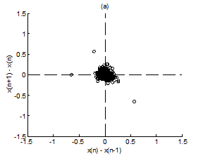
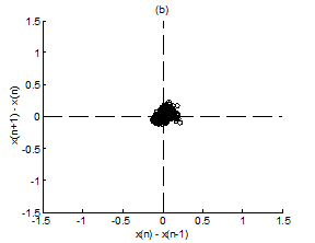
Figure 4 Scatter plot of first difference of RR intervals for Kundalini group. (A) Premeditative state. (B) Meditative state.

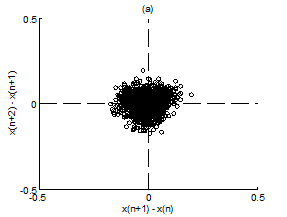
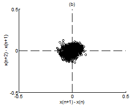
Figure 5 Scatter plot of first difference of RR intervals for Chi group. (A) Premeditative state. (B) Meditative state.

Figure 6 Plot of CTM(r) vs. r for (A) Kundalini group and (B) Chi group.

The averaged and normalized CCTM_k(r) for k=1 and 3, as functions of radius r, for premeditation and meditation states are plotted in Figure 7 and Figure 8, for Kundalini yoga and Chi group, respectively. They reflect parasympathetic and sympathetic activities during premeditation (Figure 7A & Figure 8A) and meditation (Figure 7b) and (Figure 8b), respectively. It is observed that considered individually, parasympathetic activity dominates over sympathetic activity during premeditation, while sympathetic activity dominates over parasympathetic activity during meditation in both the groups. Figure 9 and Figure 10 depict averaged and normalized sums$CCT{M}_1\left(r\right)+CCT{M}_3\left(r\right)$ and $CCT{M}_2\left(r\right)+CCT{M}_4\left(r\right)$ , both plotted as function of radius r, for premeditation and meditation states, for Kundalini yoga and Chi group, respectively. As mentioned in Sec. 2.3 they reflect low-frequency and high-frequency heart rate variation during premeditation (Figure 9A) and (Figure 10A) and meditation (Figure 9B) and (Figure 10B). It is found that irrespective of Kundalini yoga and Chi group, high-frequency heart rate variations in time domain dominate over low-frequency heart rate variations during premeditation, while low-frequency heart rate variations dominate over high-frequency heart rate variation during meditation. As a result the low-frequency-to-high-frequency ratio of heart rate variation is always lower in the premeditation state than the meditation state for a meditator. We demonstrate this finding by plotting low-frequency-to-high-frequency ratio during premeditative and meditative states for the different participants as shown in Figure 11A & 11B for Kundalini yoga and Chi group. This implies a predominance of an alternation of increases and decreases in the RR interval lengths and rapid changes in direction from interval to the next during premeditation. On the other hand, during meditation there is a predominance of progressively increasing and decreasing intervals. This can be attributed to influence of slow breathing on heart rate during meditation. One limitation of the current study is the small sample size. Factors like high variance, age differences, and differing male-to-female ratios between groups will have an impact on the results when statistical analyses are carried out on small sample sizes. Nevertheless, the results of this study provide sufficient evidence to warrant the execution of larger studies that can provide more statistically robust confirmation of the application of these methods as reliable measures of different types of meditation.

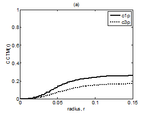
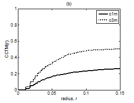
Figure 7 Plot of CCTMk(r) vs. r with k = 1 and 3 for Kundalini group (A) Premeditative state. (B) Meditative state.

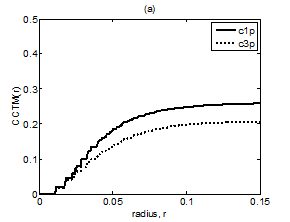
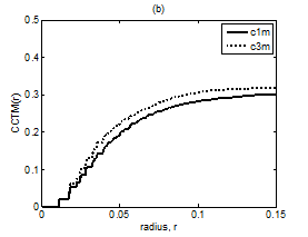
Figure 8 Plot of CCTMk(r) vs. r with k = 1 and 3 for Chi group (A) premeditative state and (B) meditative state.

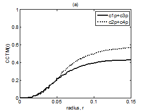
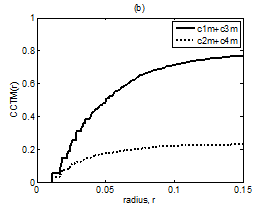
Figure 9 Plot of CCTM1(r) + CCTM3(r) vs. r and CCTM2(r) + CCTM4(r) vs. r for Kundalini group (A) premeditative state and (B) meditative state.

Figure 10 Plot of CCTM1(r) + CCTM3(r) vs. r and CCTM2(r) + CCTM4(r) vs. r for Chi group (A) premeditative state and (B) meditative state.

Figure 11 Plot of low-frequency-to-high-frequency ratio of heart rate variation for premeditative and meditative subjects of (A) Kundalini group and (B) Chi group.

In this paper, we presented two computationally simple, but efficient methods to evaluate dynamic changes in cardiac inter-beat intervals and ANS during meditation. Both Poincaré and sequence trend analysis showed lowering of complex dynamics in the RR interval series during meditation. In the Poincaré plot analysis SD2/SD1 ratio increased in the meditation state compared to the corresponding value in the premeditation state indicating a shift of the sympathovagal balance from parasympathetic towards sympathetic predominance. In the sequence trend analysis the component central tendency measures of quadrants 3 and 1 distinctly showed increased sympathetic activity and decreased parasympathetic activity during meditation and exactly the opposite during premeditation. Further, the increased low-frequency-to-high-frequency ratio in the meditation state compared to their corresponding value in the premeditation state indicates sympathetic predominance. In conclusion, it is found through both the methods that during premeditation state there is parasympathetic dominance while during meditation state there is sympathetic dominance. The results indicate that further investigation into the physiological effects of relaxation and meditation would be fruitful in increasing our understanding of the meditation and cardiac health connection.

Author declares that there is no conflicts of interest.

The author, who is also the corresponding author, is the sole contributor to this work.

1. Chinwanno W, Phawaphutanon N, Mahasarakam W, et al. Meditation in Tripitaka: Development of interpretation of meditation teaching in Theravada Buddhism in Thailand, (in Thai). Bangkok: Chulalongkorn University Press; 2000.
2. Phongsuphap S, Pongsupap Y. Analysis of heart rate variability during meditation by a pattern recognition method. Computing in Cardiology. 2011;38:197−200.
3. Lou HC, Kjaer TW, Friberg L, et al. A 15 O-H 2 O PET study of meditation and the resting state of normal consciousness. Hum Brain Mapp. 1999;7(2):98−105.
4. Travis F, Pearson C. Pure consciousness: distinct phenomenological and physiological correlates of “consciousness itself”. Int J Neurosci. 2000;100(1−4):77−89.
5. Newberg A, Alavi A, Baime M, et al. The measurement of regional cerebral blood flow during the complex cognitive task of meditation: A preliminary SPECT study. Psychiatr Res. 2001;106(2):113−122.
6. Gaylord C, Orme Johnson D, Travis F. The effects of the transcendental meditation technique and progressive muscle relaxation on EEG coherence, Stress reactivity and mental health in black adults, Int J Neurosci. 1989;46(1−2):77−86.
7. Panjwani U, Gupta HL, Singh SH, et al. Effect of Sahaja yoga practice on stress management in patients of epilepsy. Indian J Physiol Pharmocol. 1995;39(2):111−116.
8. Lee MS, Bae BH, Ryu H, et al. Changes in alpha wave and state anxiety during Chun Do Sun Bup Qi-training in trainees with open eyes. Am J Chinese Med. 1997;25(3−4):289−299.
9. Badra LJ, Cooke WH, Hoag JB, et al. Respiratory modulation of human autonomic rhythms. Am J Physiol-Heart and Circulatory Physiol. 2001;280(6):H2674−H2688.
10. Dreifus LS, Agarwal JB, Botvinick EH, et al. Heart rate variability for risk stratification of life-threatening arrhythmias. J Am Coll Cardiol. 1993;22(3):948−950.
11. Heart rate variability: standards of measurement, physiological interpretation, and clinical use. Task Force of the European Society of Cardiology and the North American Society of Pacing and Electrophysiology. Circulation. 1996;93(5):1043−1065.
12. Kheder G, Kachouri A, Messouad MB, et al. Application of a nonlinear dynamic method in the analysis of the HRV (Heart rate variability) towards clinical application: Tiresome diagnosis. Proceedings of IEEE International Conference on Information and Communication Technologies. 2006. p. 177−182.
13. Vuksanovic V, Vera gal. Nonlinear and chaos characteristics of heart period time series: Healthy aging and postural change. Auton Neurosci. 2005;121(1-2):94−100.
14. Stein PK, Reddy A. Non-linear heart rate variability and risk stratification in cardiovascular disease. Indian Pacing and Electrophysiology Journal. 2005;5(3):210−220.
15. Brien I, Hare P, Corral R. Heart rate variability in healthy subjects: effect of age and the derivation of normal ranges for test of autonomic function. Br Heart J. 1986;55(4):348−354.
16. Al-Hazimi A, Al-Ama N, Syiamic A, et al. Time domain analysis of heart rate variability in diabetic patients with and without autonomic neuropathy. Annals of Saudi Medicine. 2002;22(5−6):400−402.
17. Kleiger RE, Stein PK, Bigger JT Jr. Heart rate variability: measurement and clinical utility. Ann Noninvasive Electrocardiol. 2005;10(1):88−101.
18. Seely AJ, Macklem PT. Complex systems and the technology of variability analysis. Crit Care. 2004;8(6):R367−R384.
19. Goshvarpour A, Goshvarpour A. Chaotic Behavior of Heart Rate Signals during Chi and Kundalini Meditation. I.J. Image, Graphics and Signal Processing. 2012;2:23−29.
20. Dey A, Mukherjee S, Palit SK, et al. A new kind of dynamical pattern towards distinction of pre-meditative and meditative states through HRV. International Journal of Research and Reviews in Computer Science 2012;3(3):1611−1615.
21. Goswami DP, Tibarewala DN, Bhattacharya DK. Analysis of heart rate variability signal in meditation using second-order difference plot. Journal of Applied Physics. 2011;109:114703.
22. Luciano Bernardi, Peter Sleight, Gabriele Bandinelli, et al. Effect of rosary prayer and yoga mantras on autonomic cardiovascular rhythms: comparative study. BMJ. 2001;323:22–29.
23. Hoshiyama M, A Hoshiyama A. Heart Rate Variability Associated with Experienced Zen Meditation. Computers in Cardiology. 2008;35:569−572.
24. Matzner SA. Heart rate variability during meditation. Statistical Signal Processing ECE. 2003;510:1−4.
25. Kiran Arora AK, Kaur D, Ghay R. Impact of meditation on autonomic nervous system- A research study. International Journal of Basic and Applied Medical Sciences. 2011;1(1):144−148.
26. Goswami DP, Tibarewala DN, Bhattacharya DK. Analysis of heart rate variability signal in meditations using second-order difference plot. Journal of Applied Physics. 2011;109(11):114703.
27. De Carvalho JLA, Rocha AF, Oliveira Nascimento FA, et al. Development of a Matlab software for analysis of heart rate variability. 6th International Conference on Signal Processing. 2002;2:1488−1491.
28. Goldberger AL, Luis Amaral AN, Leon Glass, et al. PhysioBank, PhysioToolkit and PhysioNet: components of a new research resource for complex physiologic signals. Circulation. 2000;101:e215−e220.
29. Piskorski J, Guzik P. Geometry of the Poincar´e plot of RRintervals and its asymmetry in healthy adults. Physiol Meas. 2007;28(3):287–300.
30. Malliani A, Pagani M, Furlan R, et al. Individual recognition by heart rate variability of two different autonomic profiles related to posture. Circulation. 1997;96(12):4143−4145.
31. Raetz SL, Richard CA, Garfinkel A, et al. Dynamic characteristics of cardiac R-R intervals during sleep and waking states. Sleep. 1991;14(6):526−533.
32. Schechtman VL, Raetz SL, Harper RK, et al. Dynamic analysis of cardiac R-R Intervals in normal infants and in infants who subsequently succumbed to the sudden infant death syndrome. Pediatric research. 1992;31(6):606−612.
33. Abásolo D, Hornero R, Gómez, et al. Analysis of EEG background activity in Alzheimer’s disease patients with Lempel–Ziv complexity and central tendency measure. Medical Engineering and Physics. 2006;28(4):315–322.
34. Cohen ME, Hudson DL, Deedwania PC. Applying continuous chaotic modeling to cardiac signal analysis. IEEE Engineering in Medicine and Biology Magazine. 1996;15(5):97–102.
35. Kamath C. A new approach to detect congestive heart failure using Teager energy nonlinear scatter plot of RR interval series. Medical Engineering and Physics. 2012;34(7):841−848.
36. Thuraisingham RA. A Classification system to detect congestive heart failure using second-order difference plot of R-R intervals. Cardiology Research and Practice. 2009;807379:1−7.
37. Guzik P, Piskorski J, Krauze T, et al. Correlations between the Poincaré plot and conventional heart rate variability parameters assessed during paced breathing. J Physiol Sci. 2007;57(1):63–71.