This paper reports the results of an experimental study that was conducted in the laboratory of Fluid Mechanics Institute of Toulouse "IMFT". The aim of this work is to determine the velocity components over homogeneous bed roughness. The experimental design is a rectangular channel 4 m long and 0.4 m wide and 0.8m deep. The bottom has a homogeneous roughness contrast (installation of a mat). For the measurement of speed, the channel is equipped with a fast camera. In fact, the method used and developed lies in the application of a PTV particle tracking technique (Particle Tracking Velocimetry). It is a non-intrusive measurement technique to measure instantaneous speed in two-dimensional fields in stationary and unsteady flows. It involves seeding the flow through reflective particles, with the same density as the fluid, which will be lit using a lighting plan. Analysis of the results is by processing images taken by the camera using quick Matlab that is suitable for our case study. The obtained results show a depression of the maximum speed below the free surface. This behavior indicates a delay of the flow near the free surface and this is a direct consequence of the presence of secondary flows in these areas.

Keywords: free surface flow, rough bottom, experimentation, artificial canal, particle tracking velocimetry, wall parameters.

a_x: Distance between 2 roughness in the transverse direction (m)
a_y: Distance between 2 roughness in the longitudinal direction (m)
B: Width of the channel (m)
C: Roughness function
d: Displacement height of the velocity logarithmic profile (m)
D: Averaged diameter of the large-scale roughness (m)
g: the gravitational constant (m/s^-2)
h: Water depth in the channel (m)
Q: Flow rate transit (m³/s)
K: Turbulent Kinetic energy (m²/s²)
ĸ: Von Karman constant
k_s: Roughness height (m)
n: The Manning coefficient (s/m^1/3)
Re: Reynolds number $\left((v.h)/v\right)$
R²: Coefficient of correlation
S: Bed Slope
U: Longitudinal mean velocity (m/s)
u*: Friction velocity (m/s)
u*_th: Friction velocity found by the theoretical method
V: Transversal mean velocity (m/s)
W: Velocity component in the Y direction (m/s)
$\overline{u\text{'}w\text{'}}$ : Turbulent shear stress (m²/s²)
Z:  Vertical axis (m)
z₀: Hydraulic roughness (m)
$\lambda$ : Roughness density
$v$ : Kinematic viscosity (m/s²)

The free surface flows in natural and urban environments, usually occur with inhomogeneous boundary conditions because of the distribution of the bottom roughness, fixed or mobile, and/or the large deformations of the free surface for shallow currents against the bottom irregularities. In flows under load or with free surface in rectilinear channels, the wall roughness is the source of secondary flows generated by the turbulence anisotropy and the transverse variations of wall friction. In fact, in open channel flows the anisotropy of turbulence produced by the damping of velocity vertical fluctuations under the free surface has an important role and it is responsible for significant differences between flows in load and flows with free surface. Several experimental studies have been conducted to study the flow on the rough bottom. We can mention some of them: Chouaib Labiod¹ carried out experiments with a mode of placement of the bars on the channel bottom which gives a homogeneous bed roughness; Emma Florens² also carried out macro roughness experiments on the channel bottom; Zaouali Sahbi³ studied the structure and modeling of free surface flows in inhomogeneous roughness channels. Also, Cassan et al.⁴ conducted experiments with macro roughness blocks with different shapes and concentrations; the purpose of this study was to provide a stage-flow relationship for fish passage configurations. Talbi et al.⁵ conducted experiments on homogeneous and inhomogeneous rough beds to determine velocity component profiles and Reynolds stress profiles at various locations.

In this context, the present experimental study is realized; it is conducted in the Fluid Mechanics Institute of Toulouse "IMFT". In fact, in this study homogeneous bed roughness is considered in order to characterize the hydraulic resistance and the turbulent properties for large scale roughness as boulder or vegetation. The method used and developed to measure, is the PTV particle tracking technique (Particle Tracking Velocimetry). One major advantage of this technique is that the flow field structures can be examined at a prescribed instant of time in total; and by means of a fast camera, we can determine the longitudinal evolution of the average velocity fields, and Reynolds stresses$(\overline{u\text{'}w\text{'}})$ .

Many experimental correlations are available but the velocity measurements are rarely completed.^6,7 These can be linked to the difficulty of using an intrusive probe in flow with low water depth in the laboratory flume. For this purpose, the experiments conducted in the present study tried to provide other results to be useful for future simulations and scenarios.

The logarithmic rate law, for fully rough plan takes two equivalent forms, the formulation Reynolds number or on the roughness:

$\begin{array}{ccc}{\text{U}}^{\text{+}}{\text{=U/u}}^{\text{*}}{\kappa }^{\text{-1}}{\text{Ln(Z}}^{\text{+}}{\text{)+C(k}}_{\text{S}}^{\text{+}}\text{)}& {\text{Z}}^{\text{+}}{\text{=u}}^{\text{*}}\text{Z/}\nu & {\text{Z}}^{\text{+}}{\text{=u}}^{\text{*}}\text{Z/}\nu \end{array}$                                          (1)
$\begin{array}{cc}{\text{U}}^{\text{+}}\text{=}{\kappa }^{\text{-1}}{\text{ln(Z}}^{\text{*}}{\text{)+B}}_{\text{r}}{\text{(k}}_{\text{S}}^{\text{+}}\text{)}& {\text{Z}}^{\text{*}}{\text{=Z/k}}_{\text{S}}\end{array}$                                                                          (2)
${\text{B}}_{\text{r}}{\text{=C+κ}}^{\text{-1}}{\text{ln(k}}_{\text{S}}^{\text{+}}\text{)}$ (3)

The functions of the number of roughness $C\left(k_S{}^{+}\right)et{B}_r\left(k_S{}^{+}\right),$ expresses relatively universally in the asymptotic case of rough diet.

Note $K_{SS}{}^{+}$ and $K_{SR}{}^{+}$ the values of the number of roughness which respectively define upper and lower limits of fully rough regime.

The fully rough regime depends on the $K_{SR}{}^{+}$ value of the roughness number, which also depends on the roughness type. However, the constant BrR should not depend on the type of roughness and the most commonly accepted value for the work of Nikuradse⁸ is =8.5.

In summary, the expressions of $C\left(k_S{}^{+}\right)et{B}_r\left(k_S{}^{+}\right)$ corresponding are:
$K_S{}^{+}>K_{SR}{}^{+}:B_r\left(k_S{}^{+}\right)=B_{rR}=8.5$                                    (4)
$C\left(k_S{}^{+}\right)=B_{rR}–k^{-1}ln\left(k_S{}^{+}\right)$                                                (5)

The experimental device (Figure 1) is composed of a rectangular channel made of glass, open pit having length of 4m, a height equal to 0.8m and a width of B=0.4m. The slope of the channel being adjustable, and varies between 0 and 6%. Circulation loop (stable) water is provided by an electric pump providing a maximum throughput of 20 l/s. This pump delivers water through a pipe from a downstream tank from the channel to another upstream.

Figure 1 The channel and the annexes.

The control of the water level is done using a valve downstream of the channel and the flow control is done with a guillotine valve. Flow rates, Q, were measured using electromagnetic flow meters KRHONE with an accuracy of 0.5%.

On the bed, initially smooth, we stuck in the longitudinal direction of the flow equidistant roughness lurking distributed throughout the channel (Figure 2).

Figure 2 The channel bottom roughness.

Thus, we achieve a high uniform roughness background, object of our study (Figure 3). The roughness density $\lambda$  is about 24% if we consider the averaged diameter (D) of 14mm.⁹ The transversal (a_x) and longitudinal (a_y) distance between two rough elements allows defining the density as follows:
$\lambda =\frac{\pi D^2/4}{a_x{a}_y}$                                                                                            (6)

Figure 3 Geometrical description of the roughness used over the bed.

In this study, the measuring means developed and used corresponding to a particle tracking technique (Particle Tracking Velocimetry) using a fast camera (Figure 4). This is a non-intrusive measurement technique for measuring two-dimensional fields of instantaneous velocities in unsteady and steady flows. It consists in inoculating the flow study using reflective particles, having a diameter about 2mm and the same density as the fluid, which will be illuminated with an illumination plane.⁴

Figure 4 The PTV equipment’s in the laboratory of IMFT.

A fast camera (1024 * 1280 pixels) allows you to view the free surface of a pattern by ombroscopy, placed face a LED lighting system to differentiate the air from the water. The acquired image sequence sets the gray scale particles which, after treatment, will have access to the two components of the velocity vector in the plan.

Compared to other measuring methods, the PTV is an effective way to access instantly to different spatial scales of a turbulent flow in the same plane. Indeed, while the LDV, for example, requires a lot of careful movement of the equipment to obtain a high spatial resolution in a measuring plane in question, PTV provides, in the same plane, the information at the same instant in each point of space.¹⁰

A series of 5000 images is taken for each flow rate. The averaged time value is determined by calculating the averaged signal for each pixel. This enabled us to calculate a mean for the water depth in the transverse direction. The free surface is identified by the minimum signal. A mean water depth of the pattern is then derived by integrating the free surface in the longitudinal direction. The slopes of the channel tested are: S = 1 and 2%. The flow rates for each slope are respectively: Q = 5, 10, and 15 l/s.

By determining the displacement of a particle between two consecutive images, we can measure the velocity. Analysis is performed on a large number of particle detection. By grouping the measures in areas of 30 pixels, we obtain a cartography of the averaged transversely velocity field (Figure 5).

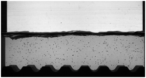
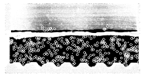
Figure 5 Experimental picture (left) for S = 1%, Q = 10l/s and particles detected in white circle (right).

The Stokes number is a dimensionless number used in fluid dynamics to study the behaviour of a particle in a fluid.¹¹ It represents the ratio between the kinetic energy of the particle to the energy dissipated by friction with the fluid.¹²

It is defined as follows:
$S_t=\frac{{\rho }^2{}_P{D}^2{}_{P}U}{\mu L_C}$ (7)

Where:
${\rho }_p$ : Density of the particle (1kg/m³)
D_p: Characteristic length of the particle (0.0008m)
U: Cinematic fluid velocity
$\mu$ : Dynamic viscosity of the fluid (10^-3kg/ m.s)
L_c: Characteristic length (m)
This number is used to determine the behaviour of a particle in a fluid encountered an obstacle and in particular whether the particle will circumvent the obstacle (if S_t<1) by following the movement of fluid or if it will percolate the obstacle (if S_t > 1).

In our case, the Stokes numbers are given in the Table 1. The Stokes number is small, so it is in a case where the particles follow the water flow.

Several tests were made to validate the measurement methodology. We worked with different frame frequency and different numbers of images per sequence (10000 and 5000 images). It appears that this is the maximum frequency given by the frequency generator which gives the most accurate results. Secondly, we choose to work with 5000 images per sequence because with 10000 images the recording and processing are slower and the accuracy is not increased by supplementary images.

In the following results, therefore we kept a number of image 5000 im/Seq, and we worked with the maximum frequency of 360 Hz. The Table 2 resumes the experimental runs in our study.

Determination of wall parameters

The formulation of the logarithmic law requires to determine the friction velocity u*, z₀ position of the origin of the logarithmic law, and a function of the roughness$C\left(K_S{}^{+}\right)or{B}_r\left(k_S{}^{+}\right)$ . In the formulation in the Reynolds number, the logarithmic law of velocity is written in effect:

$\begin{array}{cc}{\text{U}}^{\text{+}}\text{=}{\kappa }^{\text{-1}}{\text{ln(Z}}^{\text{*}}{\text{)+B}}_{\text{r}}{\text{(k}}_{\text{S}}^{\text{+}}\text{)}& {\text{Z}}^{\text{*}}{\text{=Z/k}}_{\text{S}}\end{array}$ (8)

To determine u*, z₀, B_r along the back wall we adopt, over the rough bottom, the methodology applied by Labiod.¹ Under this approach, the determination of these three parameters is done in three steps:

In a first step, we determine the pairs (u*; z₀) that check the slope of the logarithmic law with a correlation coefficient of at least 0.99, based on linear regression analysis of the relationship ${\text{U}}^{\text{+}}\to {\kappa }^{\text{-1}}{\text{u}}^{\text{*}}{\text{Ln(z+z}}_{\text{0}}\text{)}$ for each vertical velocity profile.

In a second step, we linearly extrapolate the shear stress profile -u'w' to the origin z = z₀ of the logarithmic law.

As a result, the friction velocity is directly deduced from the logarithmic law applied in the wall region, for each speed profile. This approach was adopted, also, for determining the vertical distribution of friction on the side wall.

The Figure 6 shows the determination of the wall parameters by the shear stress method and the logarithmic law method.

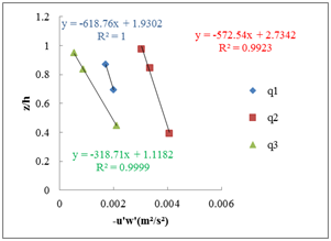
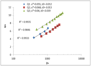
A) Method of shear stress: slope 1%            B) Method of logarithmic law: slope 1%

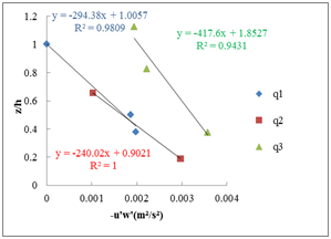
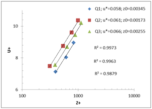
C) Method of shear stress: slope 2%           D) Method of logarithmic law: slope 2%

Figure 6 Determination of the wall parameters for the different flow rates (Q1=5 l/ s; Q2=10l/ s; Q3=15l/ s) and the different slopes; A−B) slope 1%, C−D) slope 2%.

Here is the Table 3 that summarizes the u*(m/ s) found by the various methods: The logarithmic law, the shear stress, and the theoretical method as follows:

$u_{th}^{*}=\sqrt{ghS}$ (9)

To choose the adequate values of z₀ Table 4, we proceeded by interpolation while verifying the slope of the logarithmic law with a coefficient of correlation R² always near 0.99, as well as values of u* determined from the shear stress.

We find near values of u* determined by the logarithmic law and the shear stress, while those found theoretically present a slight shift, this may be due to slope precision errors.

Dimensionless results

The figures show the dimensionless results, where u* it is the average of the ones determined by the different methods.

In this study, only the double spatially averaged profiles are presented. The transversal integration is obtained by the experimental method as explained before. The longitudinal integration is provided numerically by averaging the picture over 6 a_x.

On Figure 7, was drawn the vertical profiles of the mean longitudinal velocity, above the rough bottom, for different flow rates. It is found that more the flow rate became higher; more increases the velocity U, which is quite expected.

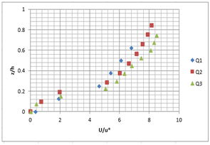
A                                                    B

Figure 7 Vertical profile of the longitudinal velocity U for the different flow rates (Q1=5 l/ s; Q2=10l/ s; Q3=15l/ s) and the different slopes; A) slope 1%, B) slope 2%.

We also note that, on these profiles, a depression of the maximum velocity below the free surface. In fact, this behavior indicates a retardation of the flow near the free surface, which is a direct consequence of the presence of secondary flows in these areas.¹

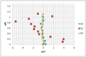
These vertical profiles confirm the in-situ and literature observations.¹³ These measurements with PTV, show that transverse velocity V (Figure 8) near the surface is lower and maximum near the rough bottom. These measures must be taken with caution as the particle detection in the area near the free surface is difficult.¹⁴

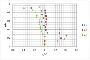
A                                                    B

Figure 8 Vertical profile of the transverse velocity V for the different flow rates (Q1=5 l/ s; Q2=10l/ s; Q3=15l/ s) and the different slopes; A) slope 1%, B) slope 2%.

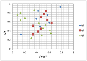
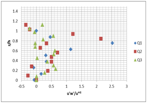
Figure 9 show that the profiles of the turbulent shear stress u'w' often exhibit deviations from the expected linear profile of parallel flow: it is the most significant sign of the secondary flows presence and their impact on transportation of longitudinal movement quantity.³

A                                                    B

Figure 9 Vertical profile of the turbulent shear stress u'w' for the different flow rates (Q1=5 l/s; Q2=10l/s; Q3=15l/s) and the different slopes; A) slope 1%, B) slope 2%.

In the wall region, the shear stress is greater at the level of the rough bottom. This is a direct effect of the roughness. Away from the wall, the situation is reversed following the adjective transport turbulence, by descendant’s flows, from low production zones (free surface) to the channel bottom (above the rough bottoms).

The influence of secondary flows on the evolution of the turbulent shear stress is well demonstrated by the momentum balance. The u'w' nonlinearity is indeed flowing developed non-parallel, a consequence of the transport amount of longitudinal movement by the secondary flows.

In our case, the maximum of turbulent kinetic energy (Figure 10) is achieved in the fluctuation zone (which is located above the rough bottom and below the free surface) because the velocity decreases and increases agitation.²

A                                                    B

Figure 10 Vertical profile of the turbulent kinetic energy K for the different flow rates (Q1=5 l/ s; Q2=10l/ s; Q3=15l/ s) and the different slopes; A) slope 1%, B) slope 2%.

Experiments in a laboratory experimental channel with a uniform roughness bottom were conducted. The technique of fast camera has been developed and used for the determination and the measurement of the velocity components. It should be noted that one advantage of the bottom roughness is to slow the flow vertical velocity. In the found results we highlight the presence of a depression of the maximum velocity below the free surface. This behavior indicates a retardation of the flow near the free surface which is a consequence of the secondary flows presence in these areas. In addition to the main objective of these experiments, which is to trace the velocity component profiles and to evaluate the methods of determining the wall parameters; these experimental measurements can subsequently be used as reference measurements for simulations or for analytical models’ validations. Other experiments with vegetated bottoms will be performed in a larger channel at the National Agronomic Institute of Tunis (INAT), to determine the effect of vegetation on the behavior characteristics.^15,16

None.

Authors declare there is no conflict of interest in publishing the article.

1. Chouaib L. Ecoulement à surface libre sur fond de rugosité inhomogène. PhD Thesis, Université de Toulouse: France; 2005. 150p.
2. Florens E. Couche limite turbulente dans les écoulements à surface libre : Etude expérimentale d’effets de macro rugosités. PhD Thesis, Université de Toulouse: France; 2010. 254p.
3. Zaouali S. Structure et modélisation d’écoulements à surface libre dans des canaux de rugosité inhomogène. PhD Thesis, Université de Toulouse: France; 2008. 177p.
4. Cassan L. Hydraulic resistance of emergent macro-roughness at large Froude numbers. Design of nature-like fish passes. Journal of Hydraulic Engineering. 2014;140(9).
5. Talbi SH, Soualmia A, Cassan L, et al. Study of Free Surface Flows in Rectangular Channel Over Rough Beds. Journal of Applied fluid mechanics. 2016;9(6):3023−3031.
6. Rice C, Kadavy K, Robinson K. Roughness of loose rock riprap on steep slopes. Journal of Hydraulic Engineering. 1998;124(2):179−185.
7. Pagliara S, Das R, Carnacina I. Flow resistance in large-scale roughness conditions. Canadian Journal of Civil Engineering. 2008;3(11):1285−1293.
8. Hiroji Nakagawa, Iehisa Nezu. Turbulence in open-channel flows. AA Balkema: Netherlands; 1993. 293p.
9. Romdhane H, Soualmia A, Cassan L, et al. Free surface flow for homogeneous bottom roughness. 4th IAHR Europe Congress at the University of Liege; 2016 July 27−29 Belgium.
10. Adamczyk AA, Rimai L. 2-Dimensional particle tracking velocimetry (PTV): Technique and image processing algorithms. Experiments in Fluids. 1988;6(6):373−380.
11. Valery, R. Thermophysical Characteristics of Nanofluids and Transport Process Mechanisms. Journal of Nanofluids. 2019;8:1−16.
12. Beg OA, Sanchez Espinoza DE, Kadir A, et al. Experimental study of improved Rheology and Lubricity of drilling fluid enhanced with nano-particles. Applied Nanoscience. 2018;8(5):1069−1090.
13. Florens E, Eiff O, Moulin F. Defining the roughness sub layer and its turbulence statistics. Exp Fluids. 2013;54:1−15.
14. Cassan L, Laurens P. Design of emergent and submerged rock-ramp fish passes. Knowl Manag Aquat Ecosyst. 2016;417(45):1−10.
15. Defina A, Bixio A. Mean flow and turbulence in vegetated open channel flow. Water resources research. 2005;41(7):1−12.
16. Luhar M, Rominger J, Nepf H. Interaction between flow, transport and vegetation spatial structure. Environ Fluid Mech. 2008;8:423−439.