
Research Article Volume 7 Issue 6
Wrapped hb-skewed laplace distribution and its application in meteorology
Jisha Varghese,
KK Jose
Department of Statistics, Mahatma Gandhi University, India
Correspondence: KK Jose, Department of Statistics, St.Thomas College, Mahatma Gandhi University, Kottayam, Kerala
Received: August 09, 2017 | Published: November 20, 2018
Citation: Varghese J, Jose KK. Wrapped hb-skewed laplace distribution and its application in meteorology. Biom Biostat Int J. 2018;7(6):525–530. DOI: 10.15406/bbij.2018.07.00255
Download PDF
Abstract
In this paper,we introduce a new circular distribution called Wrapped Holla and Bhattacharya’s (HB) Skewed Laplace distribution.We obtain explicit form for the density and derive expressions for distribution function, characteristic function and trigonometric moments. Method of maximum likelihood estimation is used for estimation of parameters. The methods are applied to a data set which consists of the wind directions of a Black Mountain ACT and compared with that of wrapped variance gamma distribution (WvG) and generalised von Mises (GvM) distribution.
Keywords: circular distribution, laplace distribution, hb skewed laplace, trigonometric moments, meteorology, wind direction
Introduction
Circular or directional data arise in different ways. The two main ways correspond to the two principal circular measuring instruments, the compass and the clock. Typical observations measured by the compass include wind directions and directions of migrating birds. Data of a similar type arise from measurements by spirit level or protractor. Typical observations measured by the clock include the arrival times (on a 24-hour clock) of patients at a casualty unit in a hospital. Data of a similar type arise as times of year or times of month of appropriate events. A circular observation can be regarded as a point on a circle of unit radius, or a unit vector (i.e. a direction) in the plane. Once an initial direction and an orientation of the circle have been chosen, each circular observation can be specified by the angle from the initial direction to the point on the circle corresponding to the observation.
Circular data are usually measured in degrees. Sometimes it is useful to measure in radians. For more details see Mardia & Jupp.1 Circular Statistics is the branch of statistics that addresses the modeling and inference from circular or directional data, i.e. data with rotating values. Many interesting circular models can be generated from known probability distributions by either wrapping a linear distribution around the unit circle or transforming a bivariate linear r.v. to its directional component. Two dimensional directions can be represented as angles measured with respect to some suitably chosen ”zero direction”. Since a direction has no magnitude, it can be conveniently represented as points on the circumference of a unit circle centered at the origin or as unit vectors connecting the origin to these points. Because of this circular representation, observations on such two dimensional directions are called circular data Jammalamadakka & Sen Guptha.2 Directional data have many unique and novel features both in terms of modeling and in their statistical treatment. In meteorology, wind directions provide a natural source of circular data. A distribution of wind directions may arise either as a marginal distribution of the wind speed and direction, or as a conditional distribution for a given speed. Other circular data arising in meteorology include the times of day at which thunderstorms occur and the times of year at which heavy rain occurs.
Recently, statisticians have shown active interest in the study of circular distribution because of their wide applicability. Jammalamadakka & Kozubowski3 discussed circular distributions obtained by wrapping the classical exponential and Laplace distributions on the real line around the circle. Rao et al.,4 derived new circular models by wrapping the well known life testing models like log normal, logistic, Weibull and extreme-value distributions. Roy & Adnan5 developed a new class of circular distributions namely wrapped weighted exponential distribution. In another work, Roy & Adnan6 explored wrapped generalized Gompertz distribution and discussed its application to Ornithology. Recently, Jacob & Jayakumar7 derived a new family of circular distribution by wrapping geometric distribution and studied its properties. Rao et al.,8 discussed the characteristics of wrapped Gamma distribution. Adnan & Roy9 derived wrapped variance Gamma distribution and showed its applicability to wind direction. Joshi & Jose10 introduced a wrapped Lindley distribution and applied it for a biological data. Recently, Jammalamadakka & Kozubowski11 introduced a general approach to obtain wrapped circular distributions through mixtures. The present paper is arranged as follows. In section 1, we give the general introduction about circular distribution. Section 2 explains the basic theory of circular distribution. Section 3 explains about the importance of Laplace distribution. In section 4, we discuss about skewed Laplace distribution. In section 5, we consider Holla and Bhattacharya’s (HB) Skewed Laplace (HBSL) distribution. In section 6, the Wrapped Holla and Bhattacharya’s (HB) Skewed Laplace (WHBSL) distribution is introduced and the probability density function (pdf) is obtained. In section 7, we derive the cumulative distribution function (cdf) and in section 8, the characteristic function and trigonometric moments are obtained. In Section 9, maximum likelihood estimation method is discussed to estimate the model parameter. In section 10, we apply the proposed model to a data on wind direction compared with that of wrapped variance gamma distribution (WvG) and generalised von Mises (GvM) distribution by using Akaike information criterion (AIC), Bayesian information criterion (BIC) and log-likelihood. Finally, Section 11 summarizes the findings.
Theory of circular distribution
A circular distribution is a probability distribution whose total probability is concentrated on the circumference of a unit circle.Since each point on the circumference represents a direction, such a distribution is a way of assigning probabilities to different directions or defining a directional distribution. The range of a circular random variable (rv)
, measured in radians, may be taken to be [0, 2
) or [-
,
). Circular distributions are essentially of two types: discrete and continuous. In continuous case, a probability density function (pdf) f(
)exists and has the following basic properties:
for any integer k.
Distribution function
One way of specifying a distribution on the unit circle is by means of its distribution function. Let f(
) be the probability density function of a continuous random variable
i.e.f(
) is a non-negative 2
periodic function such that f(
) = f(
) and
. The distribution function F(
) can be defined over any interval (
) by F(
)-F(
)=
. Suppose that an initial direction and orientation of the unit circle have been chosen (generally
direction and anticlockwise orientation). Then F(
) is defined as
obviously it holds that, F(2
) = 1.
Laplace distribution
The Laplace distribution was first introduced by Pierre Simon Laplace in 1774 and is often called the ‘first law of errors’. A continuous random variable X is said to follow classical Laplace distribution with the parameters
and
, if its pdf is given by Johnson et al.12
(1)
The random variable X following Laplace distribution (1) is denoted by
, where the constants
and
are known as the location and scale parameter respectively. The corresponding cdf is obtained as
(2)
A standard form of the pdf (1) is obtained by putting
and is given by
(3)
This form is sometimes called ‘Poisson’s first law of error’. Alternatively, the standard density function (3) is obtained by considering the transformation.
(4)
Skewed version of Laplace distribution
Skewed - Laplace distributions are considered as a generalization of the symmetric Laplace distribution. The discrete analogue of the symmetric Laplace distribution has been derived recently Kozubowski et al.,11 as in the case of normal distribution. The traditional models based on normal distribution are very often not supported by real life data in many studies because of long tails and asymmetry present in these data. The symmetric Laplace distribution(being heavier tailed than the normal) and the asymmetric Laplace distribution can account for leptokurtic and skewed data. Thus Laplace distribution is a natural, often superior alternative to the normal law. The Laplace distributions find applications in diversified fields. The classical symmetric Laplace distribution is regarded as an appropriate model in areas such as ocean engineering and fracture problems. It has also been found to be a suitable model for the formation of sand dunes. The asymmetric Laplace distributions are being used in modeling of financial data. There is a growing interest in stochastic modeling with Laplace distribution and its asymmetric extensions. The Laplace distribution is commonly encountered in image and speech compression applications. This distribution is also applicable for wind shear data, error distributions in navigation, encoding and decoding of analog signals, inventory management and quality control, astronomy and the biological and environment sciences.
In the last several decades various forms of skewed Laplace distributions have appeared in the literature. Kozubowski & Nadarajah13 studied different forms of skewed Laplace distributions. Mc Gill,14 Holla & Bhattacharya,15 Thomas Agnan & Poiraud-Casanoa,16 Fernandez & Steel17 and Yu & Zhang18 proposed different skewed Laplace distributions. Here we consider Holla and Bhattacharya’s Skewed Laplace distribution and derived its circular density function, distribution function, characteristic function and trigonometric moments.
Holla and Bhattacharya’s skewed Laplace distribution
Mc Gill14 considered distributions with the pdf given by
(5)
where
and
. These distributions are also known as the two-piece double exponential. Holla and Bhattacharya’s skewed Laplace distribution is a variation of Mc Gill’s skewed Laplace distribution studied by Holla & Bhattacharya.15 The pdf of this distribution is given by
(6)
where
,
. and
. Holla and Bhattacharya used this distribution as the compounding distribution of the expected value of a normal distribution.
The mean is obtained as
The variance is
The n
moment is
(7)
Particular case
When
, Holla and Bhattacharya’s skewed Laplace distribution reduces to classical Laplace distribution. The pdf of Holla and Bhattacharya’s skewed Laplace distribution is given by (7)
For
, (7) becomes,
It can be simplified as
where
, which is the classical Laplace distribution.
Wrapped Holla and Bhattacharya’s(HB) skewed Laplace distribution
Let X follows Holla and Bhattacharya’s skewed Laplace distribution with pdf (7).Then the wrapped Holla and Bhattacharya’s skewed Laplace random variable is defined as
, such that
[0, 2
).The pdf of the corresponding wrapped distribution is given by
(8)
According to Jammalamadakka and Kozubowski (2004, 2017), we can obtain the pdf of WHB skewed Laplace distribution as
(9)
where
[0, 2
),
,
and
The density plot for different values of the parameters are given in the following Figure 1–4.
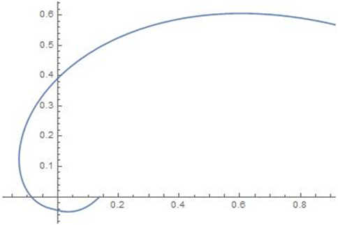

Figure 1 Density for p=0.5,
,
; Density for p=0.5,
,
.
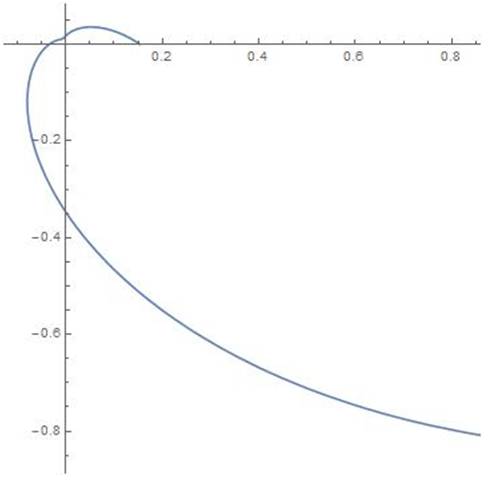
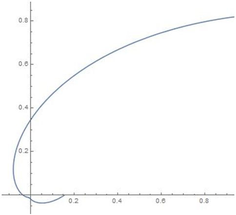
Figure 2 Density for p=0.5,
,
; Density for p=0.5,
,
.
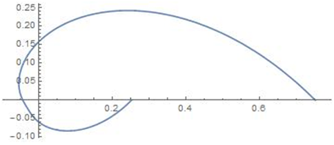
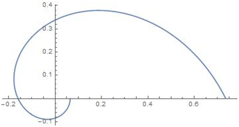
Figure 3 Density for p=0.75,
,
; Density for p=0.1,
,
.


Figure 4 Density for p=0.5,
,
; Density for p=0.5,
,
.
Distribution function
One way of specifying a distribution on the unit circle is by means of its cumulative distribution function (cdf). Let f(
) be the probability density function of a continuous random variable
. Hence f(
) is a non-negative periodic function with period 2
such that f(
) = f(
) and
. The distribution function F(
) can be defined over any interval(
) by F(
) - F(
) =
. Suppose that an initial direction and orientation of the unit circle have been chosen (generally
direction and anticlockwise orientation). Then F(
) is defined as
Obviously it follows that, F(2
) = 1
The cdf of (10) is given by
On simplification, we get
(10)
The survival function and hazard rate function can be obtained from the corresponding density function and distribution function.
Characteristic function and trigonometric moments
The characteristic function of a random angle
is the doubly-infinite sequence of complex numbers
given by
On simplification, we get
(11)
By the definition of trigonometric moments, we have
;
On simplification, we get
(12)
On simplification, we get
(13)
According to Jammalamadaka and SenGupta (2001), an alternative expression for the PDF of the wrapped distribution using the trigonometric moments is given by
(14)
Substituting the values of
and
given in (13) and (14) in (15), we get an alternative expression for the PDF of the wrapped HB skewed Laplace distribution.
Maximum likelihood estimation
In this section, the maximum likelihood estimators of the unknown parameters
of the WHB skewed Laplace distribution are derived. Let
be a random sample of size n from WHB skewed Laplace distribution, then the the likelihood function is
The log likelihood function is given by
(15)
The partial derivatives of the log likelihood with respect to p, c and
are obtained as
(16)
(17)
(18)
Inorder to estimate the parameters,we have to solve the normal equations
(19)
Since (20) cannot be solved analytically, numerical iteration technique is used to get a solution for p,c and
. One may use the nlm package in R software to get the maximum likelihood estimators (MLE) for p,c and
.
Application in meteorology
The following application shows the effectiveness of Wrapped Holla and Bhattacharya’s Skewed Laplace (WHBSL) distribution, the data wind directions comprising hourly measurements of three days at a site on Black Mountain, ACT, Australia, was reported in Dr. M.A. Cameron and discussed in Fisher.19 The main goal was to provide a regular monitoring of climate change into ACT. Climate change is the greatest threat facing the world today, wind generated electricity is one of a number of ways that we can reduce our reliance on fossil fuel-generated electricity and therefore reduce our greenhouse gas production and limit climate change. The geography and dynamics wind direction this area are important elements of climate system. This study is important given the growing evidence of the ACT climate change and biosphere to global change. The data (n= 22, degree) are as given below (Table 1).
0 |
15 |
90 |
150 |
182 |
220 |
235 |
|
240 |
245 |
250 |
255 |
265 |
270 |
280 |
285 |
300 |
315 |
330 |
335 |
340 |
345 |
|
|
Table 1 Wind direction data
Here we compute the estimates of the unknown parameters with respect to the three distributions, namely WHBSL
, WvG
and GvM
and obtain the values for loglikelihood, Akaike information criterion (AIC) and Bayesian information criterion (BIC). Table 2 provides the relevant numerical summaries for the three fits with the goodness of fit. Based on these values, we can conclude that the WHBSL
distribution is comparatively better than the other two distributions in modeling the present data.20
Distribution |
Estimates |
|
AIC |
BIC |
WHBSL |
|
97.0644 |
-188.1288 |
-188.1288 |
|
|
|
|
|
|
|
|
|
|
WVG |
|
-63.40 |
136.8 |
136.8 |
|
|
|
|
|
|
|
|
|
|
|
|
|
|
|
|
|
|
|
|
GvM |
|
-67.20 |
144.4 |
141.11 |
|
|
|
|
|
|
|
|
|
|
|
|
|
|
|
|
|
|
|
|
Table 2 Summary of fits for the wind direction data
Conclusion
In this paper, a new wrapped distribution namely Wrapped Holla and Bhattacharya’s Skewed Laplace (WHBSL) distribution is introduced and studied. The pdf and cdf of the distribution are derived and the shapes of the density function for different values of the parameters are obtained by using Mathematica. Expressions for characteristic function and trigonometric moments are derived. The alternative form of the pdf of the same distribution is also obtained using trigonometric moments. Method of maximum likelihood estimation is used for estimating the parameters. For exploring the validity of the model, we apply it to a real data set from Meteorology. The performance of the proposed model is compared with that of wrapped variance gamma distribution and generalised von Mises distribution using log-likelihood, AIC, and BIC. It is concluded that the wrapped HB Skewed Laplace distribution is a better model for the given data set than the other two distributions.
Acknowledgements
Conflict of interest
Author declares that there is no conflict of interest.
References
- Mardia KV, Jupp PE. Directional Statistics. 2nd edn, New York: Wiley; 2000.
- Jammalamadaka, S Rao, Sen Gupta A. Topics in Circular Statistics. New York: World Scientific;
- Jammalamadaka, S Rao, Kozubowski TJ. New families of wrapped distributions for modeling skew circular data. Communications in Statistics–Theory and Methods. 2004;33(9):2059–2074.
- Rao AVD, Sarma IR, Girija SVS. On wrapped version of some life testing models. Communications in Statistics–Theory and Methods. 2007;36:2027–2035.
- Roy S, Adnan MAS. Wrapped weighted exponential distributions. Statistics and Probability Letters. 2012;82:77–83.
- Roy S, Adnan MAS. Wrapped generalized Gompertz distribution: An application to Ornithology. Journal of Biometrics and Biostatistics. 2012;3(6):1013–1021.
- Jacob S, Jayakumar K. Wrapped geometric distribution: A new probability model for circular data. Journal of Statistical Theory and Applications. 2013;12(4):348–355.
- Rao AVD, Sarma IR, Girija SVS. On characteristics of wrapped gamma distribution. IRACST – Engineering Science and Technology: An International Journal (ESTIJ). 2013;3(2):228–232.
- Adnan MAS, Roy S. Wrapped variance gamma distribution with an application to wind direction. Journal of Environmental Statistics. 2014;6(2):1–10.
- Joshi S, Jose KK. Wrapped Lindley Distribution. Communications in Statistics– Theory and Methods. 2017;47(5):1013–1021.
- Kozubowski TJ, Podgorski K. Asymmetric Laplace laws and modeling financial data. Math Comput Model. 2001;34:1003–1021.
- Johnson NL, Kotz S, Balakrishnan N. Continuous Univariate Distributions. 2nd Singapore: John Wiley Sons (Asia) Pvt. Ltd; 2001.
- Kozubowski TJ, Nadarajah S. Multitude of Laplace Distributions. Stat Papers. 2001;
- McGill WJ. Random fluctuations of response rate. Psychometrika. 1962;27:3–17.
- Holla MS, Bhattacharya SK. On a compound Gaussian distribution. Ann Ins Stat Math. 1968;20:331–336.
- Poiraud Casanoa S, Thomas Agnan C. About monotone regression quantiles. Stat Probab Lett. 48(1):101–104.
- Fernandez C, Steel MFJ. On Bayesian modeling of fat tails and skewness. J Am Stat Assoc. 1998;93:359–371.
- Yu K, Zhang J. A three–parameter asymmetric Laplace distribution and its extension. Commun Stat Theory Methods. 2005;34:1867–1879
- Fisher NI. Statistical Analysis of Circular data. Melboume: Cambridge University Press;
- Jammalamadaka, S Rao, Kozubowski TJ. A General Approach for Obtaining Wrapped Circular Distributions via Mixtures. Sankhya : The Indian Journal of Statistics. 2017;33(9):2059–2074.

©2018 Varghese, et al. This is an open access article distributed under the terms of the,
which
permits unrestricted use, distribution, and build upon your work non-commercially.


