Stability within family of Pareto models

doi:10.15406/bbij.2018.07.00207

eISSN: 2378-315X

Biometrics & Biostatistics International Journal

Research Article Volume 7 Issue 3

Stability within family of Pareto models

Mariam Zahid,¹

Verify Captcha

Regret for the inconvenience: we are taking measures to prevent fraudulent form submissions by extractors and page crawlers. Please type the correct Captcha word to see email ID.

Shakila Bashir²

¹Department of Statistics, Kinnaird College for Women, Pakistan
²Department of Statistics, Forman Christian College, Pakistan

Correspondence: Mariam Zahid, Department of Statistics, Kinnaird College for Women, Near Canal bank Jail Road, Lahore, Pakistan

Received: April 16, 2018 | Published: May 9, 2018

Citation: Zahid M, Bashir S. Stability within family of Pareto models. Biom Biostat Int J. 2018;7(3):177–186. DOI: 10.15406/bbij.2018.07.00207

Download PDF

Abstract

Transmutation technique is applied to extend the workability and flexibility of weighted Pareto distribution. A weighted probability distribution improves precision for predictability and transmuting the same produces a better model for data fitting. Various statistical properties including moments and quantiles, reliability analysis, mean deviation, order statistics and record values of transmuted weighted Pareto (TWP) distribution are studied. The parameters of the distribution are evaluated using Maximum Likelihood Estimation (MLE). Application study compares different Pareto models to reveal the stability between them. A simulation analysis is also performed.

Keywords: weighted Pareto distribution, moments, reliability analysis, record values, MLE

Introduction

The goal of a probability distribution is to fit maximum data sets with utmost precision and minimum variance so that their behavior can be modeled and predicted. The existing distributions can be made more precise and useful for a wider spectrum of values by applying new techniques such as transmutation.

Pareto distribution was developed by Vilfredo Pareto. This distribution was meant to show the apportionment of income to the population. However, the purpose of the distribution is not restricted to income evaluations only; it uses the precept which requires the data to have a small to large proportion for example, the meteor showers on Earth. Fisher¹ introduced the concept of weighted distributions by highlighting the idea of need for surety of occurrence of event. Zelen² studied weighted distributions and delineated the methodology required to formulate a weighted distribution using cell kinetics. A weighted distribution is found using

$f^{w} (x; θ) = \frac{x^{k} . f (x; θ)}{μ_{k}^{'}}$ $f^{w} (x; θ) = \frac{x^{k} . f (x; θ)}{μ_{k}^{'}}$ (1)

Where $E [w (x)] = μ_{k}^{'}$ $E [w (x)] = μ_{k}^{'}$ . To derive transmuted weighted Pareto distribution, the weighted form used has k=1. Weighted distribution introduces the surety of occurrence of an event and hence can be considered a vital requisite for all probability distributions.

Transmuting a distribution means that a distribution is elaborated by adding more variables in effort to optimize its adaptability towards data. The Quadratic Rank Transmutation (QRT) technique uses an established formula to derive the new distribution.³ Transmutation, thus, can be carried out using the following relations:

$f (x) = g (x) [(1 + λ) - 2 λ G (x)]$ $f (x) = g (x) [(1 + λ) - 2 λ G (x)]$ (2)

$F (x) = (1 + λ) G (x) - λ {[G (x)]}^{2}$ $F (x) = (1 + λ) G (x) - λ {[G (x)]}^{2}$ (3)

Equation (2) and (3) give the formula that can be used to derive the pdf and cdf for the transmuted distribution. g(x) represents the pdf and G(x) is the cdf of the parent distribution and $λ \subset [- 1, 1]$ $λ \subset [- 1, 1]$ . For $λ = 0$ $λ = 0$ , the transmuted model changes back to the parent model.

Transmutation technique has been proven very successful in bringing out some useful distributions. Dar et al.⁴ studied the transmuted weighted exponential distribution. Shahzad et al.⁵ transmuted the Singh-Maddla distribution. Nasser et al.⁶ found useful results for transmuted Weibull Logistic distribution. Ashour & Eltehiwy⁷ studied the transmuted exponentiated Lomax distribution. Aryal & Tsokos⁸ found that transmuting a distribution helps in advancement of a distribution. Aryal⁹ found that new generalizations of distributions help in extending the study. Khan et al.¹⁰ derived transmuted Kumaraswamy distribution and concluded that for statistical significance of model adequacy the transmuted distribution lead to a better fit than Kumaraswamy distribution. Transmutation studies have gained attention because of their ability to generate new flexible distributions that can help fit data with more precision.

In this paper weighted Pareto distribution is transmuted. Various statistical properties of the new distribution are studied including moments, quantiles, moment generating function (MGF), Bonferroni and Lorenz curves, reliability analysis, order statistics, record values and parameter estimation. Application study compares different Pareto models to see if there is stability between them.

Transmuted weighted pareto distribution

Mir & Ahmad¹¹ derived the weighted Pareto distribution among some other weighted distributions. The pdf and cdf of the weighted Pareto distribution are given below:

$f^{w} = α^{β - 1} x^{- β} (β - 1)$ $f^{w} = α^{β - 1} x^{- β} (β - 1)$ (4)

$F^{w} = 1 - α^{β - 1} x^{1 - β}$ $F^{w} = 1 - α^{β - 1} x^{1 - β}$ (5)

Here, α is the scale parameter and β is the shape parameter such that α>0 and β>1. These are the main results for the weighted Pareto distribution that will subsequently be transmuted to form a new distribution called the transmuted weighted Pareto distribution (TWP). Equations (2), (4) and (5) are used to find the pdf of the transmuted weighted Pareto distribution:

$f_{T W P} (x; α, β, λ) = (α^{β - 1} x^{- β} (β - 1)) [1 - λ + 2 λ α^{β - 1} x^{1 - β}]$ $f_{T W P} (x; α, β, λ) = (α^{β - 1} x^{- β} (β - 1)) [1 - λ + 2 λ α^{β - 1} x^{1 - β}]$ (6)

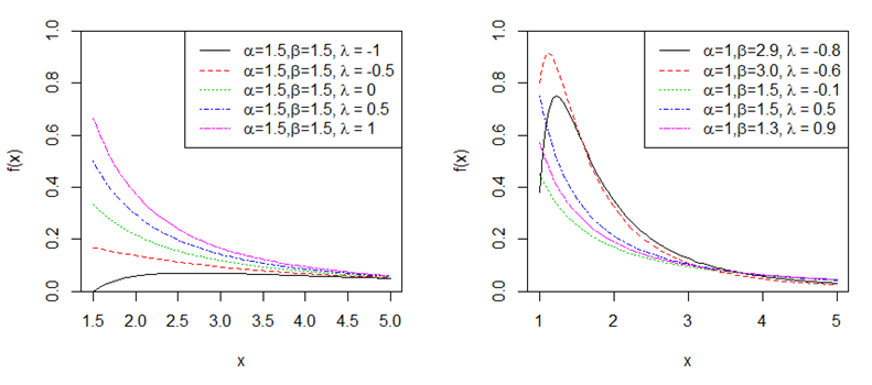
Where, $α < x < \infty, α > 0 a n d β > 1$ $α < x < \infty, α > 0 a n d β > 1$ . The graphs of the pdf of transmuted weighted Pareto distribution (TWP) are plotted to show the shape of the distribution (Figure 1).

Figure 1 Graphs of pdf of TWP distribution with different values of α, β and λ.

The graph in Figure 1 (left) uses different values for λ with constant α and β values to show how the new variable impacts the shape of the distribution. Values used for λ are -1, -0.5, 0, 0.5 because $λ \subset [- 1, 1]$ $λ \subset [- 1, 1]$ . On the other hand, graph in Figure 1 (right) shows different combinations of all the variables involved to see the changes brought by each variable. Equations (3), (4) and (5) are used to find the cdf for the transmuted weighted Pareto distribution:

$F_{T W P} (x; α, β, λ) = 1 + α^{β - 1} x^{1 - β} (λ - 1) - λ α^{2 (β - 1)} x^{2 (1 - β)}$ $F_{T W P} (x; α, β, λ) = 1 + α^{β - 1} x^{1 - β} (λ - 1) - λ α^{2 (β - 1)} x^{2 (1 - β)}$ (7)

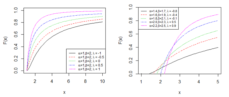
where $λ \subset [- 1, 1]$ $λ \subset [- 1, 1]$ and β>1. The cdf is graphically presented in Figure 2.

Figure 2 Graph of cdf of TWP distribution with different α, β and λ values, it shows the cdf with different λ values with constant α and β values (left) and different combinations of α, β and λ values (right).

Moments and other derived measures

This section looks deeper into the distribution by exploring its moments and other properties.

Moment generating function

The moment generating function of the transmuted weighted Pareto distribution is given by:

$M_{x} (t) = E [e^{t x}] = \infty \int 0 e^{t x} f (x) d x$ $M_{x} (t) = E [e^{t x}] = \int_{0}^{\infty} e^{t x} f (x) d x$

$= \infty \int 0 (1 + t x + \frac{t^{2} x^{2}}{2!} + \dots + \frac{t^{n} x^{n}}{n!} + \dots) f (x) d x$ $= \int_{0}^{\infty} (1 + t x + \frac{t^{2} x^{2}}{2!} + \dots + \frac{t^{n} x^{n}}{n!} + \dots) f (x) d x$

$= \infty \sum i = 0 \frac{t^{i} E (X^{i})}{i!}$ $= \sum_{i = 0}^{\infty} \frac{t^{i} E (X^{i})}{i!}$

$= \infty \sum i = 0 \frac{t^{i}}{i!} \frac{(β - 1) α^{i} [2 (β - 1) - i λ - i]}{(1 - β + i) (2 - 2 β + i)}$ $= \sum_{i = 0}^{\infty} \frac{t^{i}}{i!} \frac{(β - 1) α^{i} [2 (β - 1) - i λ - i]}{(1 - β + i) (2 - 2 β + i)}$ (8)

Moments

Moments are defining characteristics of a distribution; the moments for TWP distribution are presented in this section. The rth moment of the TWP distribution, with a random variable X, will be:

$m_{r}^{'} = E (X^{r}) = (β - 1) \frac{(λ α^{r} r - 2 λ α^{r} r - 2 α^{r} + 2 α^{r} β - α^{r} r)}{(r - β + 1) (2 - 2 β + r)}$ $m_{r}^{'} = E (X^{r}) = (β - 1) \frac{(λ α^{r} r - 2 λ α^{r} r - 2 α^{r} + 2 α^{r} β - α^{r} r)}{(r - β + 1) (2 - 2 β + r)}$ (9)

Result in eq. (9) could be used to derive moments by putting in different values for r.

$m_{1}^{'} = E (X^{1}) = (β - 1) [\frac{α (2 β - λ - 3)}{(2 - β) (3 - 2 β)}]$ $m_{1}^{'} = E (X^{1}) = (β - 1) [\frac{α (2 β - λ - 3)}{(2 - β) (3 - 2 β)}]$ (10)

$m_{2}^{'} = E (X^{2}) = (β - 1) [\frac{α^{2} (β - 2 - λ)}{(3 - β) (2 - β)}]$ $m_{2}^{'} = E (X^{2}) = (β - 1) [\frac{α^{2} (β - 2 - λ)}{(3 - β) (2 - β)}]$ (11)

$m_{3}^{'} = E (X^{3}) = (β - 1) [\frac{α^{3} (2 β - 5 - 3 λ)}{(4 - β) (5 - 2 β)}]$ $m_{3}^{'} = E (X^{3}) = (β - 1) [\frac{α^{3} (2 β - 5 - 3 λ)}{(4 - β) (5 - 2 β)}]$ (12)

$m_{4}^{'} = E (X^{4}) = (β - 1) [\frac{α^{4} (β - 3 - 2 λ)}{(5 - β) (3 - β)}]$ $m_{4}^{'} = E (X^{4}) = (β - 1) [\frac{α^{4} (β - 3 - 2 λ)}{(5 - β) (3 - β)}]$ (13)

First moment about origin is the mean of the distribution. Likewise, other higher moments can be used to find the variance, skewness, kurtosis etc.

Variance and coefficient of variation of the TWP distribution are given below:

$var (X) = E (X^{2}) - {[E (X)]}^{2}$ $var (X) = E (X^{2}) - {[E (X)]}^{2}$

$= \frac{α^{2} (2 λ β^{3} + λ^{2} β^{3} - 4 β^{3} + 16 β^{2} - 5 λ β^{2} - 5 λ^{2} β^{2} + 3 λ β + 7 λ^{2} β - 21 β + 9 - 3 λ^{2})}{{(2 - β)}^{2} {(3 - 2 β)}^{2} (3 - β)}$ $= \frac{α^{2} (2 λ β^{3} + λ^{2} β^{3} - 4 β^{3} + 16 β^{2} - 5 λ β^{2} - 5 λ^{2} β^{2} + 3 λ β + 7 λ^{2} β - 21 β + 9 - 3 λ^{2})}{{(2 - β)}^{2} {(3 - 2 β)}^{2} (3 - β)}$ (14)

$C V_{T W P} (X) = \frac{\sqrt{V a r (X)}}{E (X)}$

$= \frac{α (2 - β) (3 - 2 β) \sqrt{(\begin{array}{l} 2 λ β^{3} + λ^{2} β^{3} - 4 β^{3} + 16 β^{2} - 5 λ β^{2} \\ - 5 λ^{2} β^{2} + 3 λ β + 7 λ^{2} β - 21 β + 9 - 3 λ^{2} \end{array})}}{(2 - β) (3 - 2 β) (β - 1) [α (2 β - λ - 3)] \sqrt{(3 - β)}}$ (15)

Skewness and Kurtosis of the TWP distribution reveal information about symmetry and tail of the distribution respectively.

$S k e w n e s s_{T W P} (X) = \frac{m_{3}}{{[V a r (X)]}^{\frac{3}{2}}}$ (16)

where,

$\begin{array}{l} m_{3} = \frac{(β - 1) α^{3} (2 β - 5 - 3 λ)}{(4 - β) (5 - 2 β)} - \frac{3 α^{3} (2 β - λ - 3) (β - 2 - λ) {(β - 1)}^{2}}{(2 - β) (3 - 2 β) (3 - β)} \\ + \frac{2 α^{3} {(β - 1)}^{3} (2 β - λ - 3)}{{(2 - β)}^{3} {(3 - 2 β)}^{3}} \end{array}$

$K u r t o s i s_{T W P} (X) = \frac{m_{4}}{{[V a r (X)]}^{2}}$ (17)

where,

$\begin{array}{l} m_{4} = (β - 1) [\frac{α^{4} (β - 3 - 2 λ)}{(5 - β) (3 - β)}] - \frac{4 α^{4} {(β - 1)}^{2} (2 β - λ - 3) (2 β - 5 - 3 λ)}{(2 - β) (3 - 2 β) (4 - β) (5 - 2 β)} \\ + \frac{6 α^{4} {(β - 1)}^{3} {(2 β - λ - 3)}^{2} (β - 2 - λ)}{{(2 - β)}^{3} {(3 - 2 β)}^{2} (3 - β)} - \frac{3 {(β - 1)}^{4} α^{4} {(2 β - λ - 3)}^{4}}{{(2 - β)}^{4} {(3 - 2 β)}^{4}} \end{array}$

Quantiles

The qth quantile of the TWP distribution is found to be

$x_{q} = {\frac{α^{- 2 β} [α^{β + 1} \sqrt{{(1 + λ)}^{2} - 4 λ q} - (1 - λ) α^{β + 1}]}{2 λ}}^{\frac{1}{1 - β}}$ (18)

The median of the TWP can thus be found by putting q=0.5

$x_{0.5} = {\frac{α^{- 2 β} [α^{β + 1} \sqrt{λ^{2} + 1} - (1 - λ) α^{β + 1}]}{2 λ}}^{\frac{1}{1 - β}}$ (19)

To make skewness and kurtosis yield better results, these measures could be derived using quantiles. The original skewness and kurtosis show infinite measure for heavy-tailed distributions making it less informative. The Bowleys skewness derived as the earliest skewness measure uses average of quartiles minus the median, divided by one half interquartile ranges.

$B = \frac{Q_{3} + Q_{1} - 2 Q_{2}}{Q_{3} - Q_{1}} = \frac{Q (3 / 4) + Q (1 / 4) - 2 Q (2 / 4)}{Q (3 / 4) - Q (1 / 4)}$

For kurtosis, Moors kurtosis uses octiles to make it a better measure.

$M = \frac{(E_{3} - E_{1}) + (E_{7} - E_{5})}{E_{6} - E_{2}} = \frac{Q (3 / 4) - Q (7 / 8) - Q (5 / 8)}{Q (6 / 8) - Q (2 / 8)}$

Bonferroni and Lorenz curves

Bonferroni and Lorenz curves are important for reliability studies. The curves for the function, F(x)=p, are given by:

$B (p) = \frac{1}{p μ_{1}^{'}} \int_{0}^{q} x f (x) d x$ , $L (p) = p B (p) = \frac{1}{μ_{1}^{'}} \int_{0}^{q} x f (x) d x$ , where $q = F^{- 1} (p)$ , $F (x) = p, 0 \leq p \leq 1$

Hence, the Bonferroni and Lorenz curves for TWP respectively are

$B (p) = \frac{1}{p {(β - 1) [\frac{α (2 β - λ - 3)}{(2 - β) (3 - 2 β)}]}} (β - 1) [\begin{array}{l} \frac{(α^{β - 1} q^{2 - β} - α)}{2 - β} (1 - λ) \\ + \frac{2 λ (α^{2 β - 2} q^{3 - 2 β} - α)}{3 - 2 β} \end{array}]$ (20)

$L (p) = \frac{1}{(β - 1) [\frac{α (2 β - λ - 3)}{(2 - β) (3 - 2 β)}]} (β - 1) [\begin{array}{l} \frac{(α^{β - 1} q^{2 - β} - α)}{2 - β} (1 - λ) \\ + \frac{(2 λ (α^{2 β - 2} q^{3 - 2 β} - α))}{3 - 2 β} \end{array}]$ (21)

Mean deviation and averages

Mean deviation gives the mean of the absolute deviations from its mean value. Thus, the mean deviation of TWP distribution is calculated as

$\begin{array}{l} M D_{T W P} = 2 μ [1 + (α^{β - 1} μ^{1 - β}) (λ - 1) - λ α^{2 (β - 1)} μ^{2 (1 - β)}] \\ - 2 (β - 1) [\frac{α^{β - 1} μ^{2 - β} - α - λ α^{β - 1} μ^{2 - β}}{(2 - β)} + \frac{2 λ α^{2 (β - 1)} μ^{3 - 2 β} - 2 λ α}{3 - 2 β}] \end{array}$ (22)

Harmonic Mean of TWP:

$H M_{T W P} = \frac{β - 2 β^{2}}{(β - 1) (α^{- 1} - 2 β α^{- 1} - λ α^{- 1})}$ (23)

Geometric mean of TWP:

$G M_{T W P} = \prod_{i = 1}^{n} [(β - 1) (\frac{n α^{\frac{1}{n}} λ - n α^{\frac{1}{n}}}{1 - n β + n} - \frac{2 n λ α^{\frac{1}{n}}}{2 n - 2 β n + 1})]$ (24)

Reliability analysis

The reliability analysis involves the evaluation of various processes that assess the quality of life of the data for a time (t).

Reliability function

The reliability function for the TWP distribution tells about the length of life up to a time (t) and thus is an important characteristic to study.

$R_{T W P} (t) = α^{β - 1} t^{1 - β} (1 - λ + λ α^{β - 1} t^{1 - β})$ (25)

Hazard rate

The hazard rate tells about the rate of failure of an item. It predicts the end of its life and can be calculated as follows:

$h_{T W P} (t) = \frac{(β - 1) (1 - λ + 2 λ α^{β - 1} t^{1 - β})}{(t - λ t + λ α^{β - 1} t^{2 - β})}$ (26)

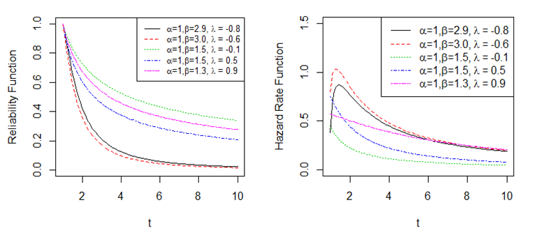
Figure 3 shows the reliability function and hazard rate function graphically. The graph uses different combinations of α, β and λ values to show a decreasing trend of the function (Figure 3).

Figure 3 Reliability and Hazard rate function graphs with different α, β and λ values.

Reversed hazard rate function

Reversed hazard rate comes handy when the time is measured in a reversed manner; therefore, it is tabulated to cover for an occurrence of that sort.

$r_{T W P} (t) = \frac{(β - 1) α^{β - 1} t^{- β} (1 - λ + 2 λ α^{β - 1} t^{1 - β})}{1 + α^{β - 1} t^{1 - β} (λ - 1) - λ α^{2 (β - 1)} t^{2 (1 - β)}}$ (27)

Cumulative hazard rate

Cumulative hazard rate combines all risks that were faced up to a time, t, and this accumulation is referred to as cumulative hazard rate.

$C H R_{T W P} (t) = - \log [λ α^{2 (β - 1)} t^{2 (1 - β)} - α^{β - 1} t^{1 - β} (λ - 1)]$ (28)

Order statistics

It is important to study the range of the probability distribution and to serve the need for range; minimum and maximum pdf’s for the TWP distribution are derived. Most commonly, the pdf for the jth order statistic is used, and is thus derived below

$f_{X_{(j)}} (x_{(j)}) = \frac{n!}{(j - 1)! (n - j)!} f_{X} (x) {[F_{X} (x)]}^{j - 1} {[1 - F_{X} (x)]}^{n - j}$

$\begin{array}{l} = \frac{n!}{(j - 1)! (n - j)!} [(α^{β - 1} x_{(j)}^{- β} (β - 1)) (1 - λ + 2 λ α^{β - 1} x_{(j)}^{1 - β})] \\ {[1 + α^{β - 1} x_{(j)}^{1 - β} (λ - 1) - λ α^{2 (β - 1)} x_{(j)}^{2 (1 - β)}]}^{j - 1} {[α^{β - 1} x_{(j)}^{1 - β} (1 - λ) + λ α^{2 (β - 1)} x_{(j)}^{2 (1 - β)}]}^{n - j} \end{array}$ (29)

Order statistics, useful for reliability studies, provide the 1st and nth order pdf for TWP distribution

$f_{(1)} (x_{(1)}) = n {[1 - F (x_{(1)})]}^{n - 1} f (x_{(1)})$

$= n {[α^{β - 1} x_{(1)}^{1 - β} (1 - λ) + λ α^{2 (β - 1)} x_{(1)}^{2 (1 - β)}]}^{n - 1} [(α^{β - 1} x_{(1)}^{- β} (β - 1)) (1 - λ + 2 λ α^{β - 1} x_{(1)}^{1 - β})]$ (30)

$f_{(n)} (x_{(n)}) = n {[F (x_{(n)})]}^{n - 1} f (x_{(n)})$

$\begin{array}{l} = n {[1 + α^{β - 1} x_{(n)}^{1 - β} (λ - 1) - λ α^{2 (β - 1)} x_{(n)}^{2 (1 - β)}]}^{n - 1} \\ \times [(α^{β - 1} x_{(n)}^{- β} (β - 1)) (1 - λ + 2 λ α^{β - 1} x_{(n)}^{1 - β})] \end{array}$ (31)

The joint pdf for X(i) and X(j) is also found for the TWP distribution

$\begin{array}{l} f_{X_{(i)}, X_{(j)}} (u, v) = \frac{n!}{(i - 1)! (j - 1 - i)! (n - j)!} f_{X} (u) f_{X} (v) {[F_{X} (u)]}^{i - 1} \\ \times {[F_{X} (v) - F_{X} (u)]}^{j - 1 - i} {[1 - F_{X} (v)]}^{n - j} \end{array}$

$\begin{array}{l} = \frac{n!}{(i - 1)! (j - 1 - i)! (n - j)!} [(α^{β - 1} u^{- β} (β - 1)) (1 - λ + 2 λ α^{β - 1} u^{1 - β})] \\ \times [(α^{β - 1} v^{- β} (β - 1)) (1 - λ + 2 λ α^{β - 1} v^{1 - β})] {[1 + α^{β - 1} u^{1 - β} (λ - 1) - λ α^{2 (β - 1)} u^{2 (1 - β)}]}^{i - 1} \\ \times {[α^{β - 1} v^{1 - β} (λ - 1) - λ α^{2 (β - 1)} v^{2 (1 - β)} + α^{β - 1} u^{1 - β} (1 - λ) + λ α^{2 (β - 1)} u^{2 (1 - β)}]}^{j - 1 - i} \\ \times {[α^{β - 1} v^{1 - β} (1 - λ) + λ α^{2 (β - 1)} v^{2 (1 - β)}]}^{n - j} \end{array}$ (32)

Random number generation and parameter estimation

Random number generation

The inversion method is used to generate random numbers for the TWP distribution

$1 + α^{β - 1} x^{1 - β} (λ - 1) - λ α^{2 (β - 1)} x^{2 (1 - β)} = u$

Here, $u ~ U (0, 1)$ . After calculation, result for x is

$x = {\frac{α^{- 2 β} [α^{β + 1} \sqrt{λ^{2} - 4 λ u + 2 λ + 1} - (1 - λ) α^{β + 1}]}{2 λ}}^{\frac{1}{1 - β}}$ (33)

Equation (33) can be used to get random numbers when the parameters α, β and λ are known.

Method of moments

One of the techniques for parameter estimation is to use method of moments. This process uses moments of the distribution to estimate parameters. Since there are three parameters, there will be three equations:

$\hat{β} = \frac{5 \hat{α} n + \hat{α} \hat{λ} n - 7 \sum_{i = 1}^{n} x_{i} + \sqrt{\begin{array}{l} {\hat{α}}^{2} n^{2} + 2 {\hat{α}}^{2} \hat{λ} n^{2} + {\hat{α}}^{2} {\hat{λ}}^{2} n^{2} + 2 \hat{α} \sum_{i = 1}^{n} x_{i} n \\ - 6 \hat{α} \sum_{i = 1}^{n} x_{i} \hat{λ} n + \sum_{i = 1}^{n} x_{i}^{2} \end{array}}}{2 (2 \hat{α} n - 2 \sum_{i = 1}^{n} x_{i})}$ (34)

$\hat{λ} = \frac{\sum_{i = 1}^{n} x_{i}^{2} {\hat{β}}^{2} - 5 \sum_{i = 1}^{n} x_{i}^{2} \hat{β} + 6 \sum_{i = 1}^{n} x_{i}^{2} - {\hat{β}}^{2} {\hat{α}}^{2} n + 3 \hat{β} {\hat{α}}^{2} n - 2 {\hat{α}}^{2} n}{{\hat{α}}^{2} n (1 - \hat{β})}$ (35)

$\hat{α} = \sqrt[3]{\frac{20 \sum_{i = 1}^{n} x_{i}^{3} - 13 \sum_{i = 1}^{n} x_{i}^{3} \hat{β} + 2 \sum_{i = 1}^{n} x_{i}^{3} {\hat{β}}^{2}}{n (5 + 2 {\hat{β}}^{2} + 3 \hat{λ} - 7 \hat{β} - 3 \hat{β} \hat{λ})}}$ (36)

Equations (34), (35) and (36) express the parameters; they can be further solved simultaneously to get cleaner expressions for the parameters.

Maximum likelihood estimation

Widely used technique for evaluating the parameters of the distribution is that of Maximum Likelihood Estimation technique. If $x_{1}, x_{2}, \dots, x_{n}$ is a random sample of size n from the TWP distribution then its log-likelihood function will be:

$L = \prod_{i = 1}^{n} f_{T W P} (x_{i}; α, β, λ) = {(β - 1)}^{n} (α^{n (β - 1)} \prod_{i = 1}^{n} x_{i}^{- β}) \prod_{i = 1}^{n} [(1 - λ + 2 λ α^{β - 1} x^{1 - β})]$

Using LL=ln L, log-likelihood function is derived

$L L = n \ln (β - 1) + n (β - 1) \ln α - β \sum_{i = 1}^{n} \ln x_{i} + \sum_{i = 1}^{n} \ln [(1 - λ + 2 λ α^{β - 1} x^{1 - β})]$ (37)

To estimate the parameters, equation (37) is differentiated with respect to β and λ and put equal to zero so as to get the respective parameters.

$\frac{\partial L L}{\partial β} = \frac{n}{β - 1} + n \ln α - \sum_{i = 1}^{n} \ln x_{i} + \sum_{i = 1}^{n} \frac{2 α^{β - 1} \ln α λ x_{i}^{1 - β} - 2 α^{β - 1} λ x_{i}^{1 - β} \ln (x_{i})}{(2 α^{β - 1} λ x_{i}^{1 - β} - λ + 1)}$ (38)

$\frac{\partial L L}{\partial λ} = \sum_{i = 1}^{n} \frac{2 α^{β - 1} x_{i}^{1 - β} - 1}{(1 - λ + 2 λ α^{β - 1} x_{i}^{1 - β})}$ (39)

For TWP distribution $x \geq α$ , α is the lower limit for this distribution so the maximum likelihood estimate of α will be the first statistic value i.e., $x_{(1)}$ . The log-likelihood function is numerically maximised by using the R software.

Simulation

Simulation can help in understanding the data sets for the particular distribution. Inverse CDF technique is used to simulate the data set in R. The values used for parameters are α=1, β=6 and λ=-0.2. A data set of size 100 is thus simulated for the TWP distribution (Table 1).

Data generated for α=1, β=3 and λ=-0.2
2.171301	2.469904	3.627952	4.122543	2.290153
1.961311	2.02465	2.788962	1.912685	2.237079
1.993091	2.611573	2.926888	2.658368	2.705542
2.050194	2.19487	2.333488	2.010353	2.462991
4.240425	2.054078	2.150241	2.836084	3.139823
3.276202	3.642714	1.914709	2.589984	1.980117
2.079828	2.081706	1.925856	1.989657	1.95235
3.188533	3.776208	2.161587	3.04785	2.287527
1.908391	1.909436	2.133601	1.945302	2.128175
2.208188	2.512261	2.831646	1.927698	2.205562
2.107547	2.102916	2.061781	2.129319	1.963237
2.142851	1.952253	2.75405	2.385384	2.056045
2.490634	1.987443	2.111349	2.256456	3.406278
2.197887	1.921594	3.08898	2.598769	2.323328
2.2008	2.32725	3.405701	2.567741	2.850449
1.931747	1.956453	2.343114	2.214165	2.446729
2.566559	1.917651	2.910597	2.54337	2.346076
1.959292	1.939467	2.359965	2.056514	2.491718
3.358692	2.762751	2.22607	2.009319	3.075688
2.161866	1.906318	2.630087	2.90743	3.515726

Table 1 Results from the simulation study of the TWP distribution

The data given above is used to estimate parameters for the distribution. Estimated values are given in Table 2.

Model	Estimates	Standard Error
Transmuted Weighted Pareto	$\begin{array}{l} \hat{β} = 5 .695927 \\ \hat{λ} = - 0 .109770 \\ \hat{α} = \min (x) = 1 .906318 \end{array}$	0.681109 0.241365

Table 2 Estimated values of parameters for TWP distribution

The variance covariance matrix for the TWP distribution with the above data will be: $| \begin{matrix} 0 .4639094 & -0 .12210893 \\ -0 .12210893 & 0 .05825721 \end{matrix} |$

This shows that the variance of MLE of β and λ are Var $(\overset{⌢}{β})$ = $0 .4639094$ and Var $(\overset{⌢}{λ})$ = $0 .05825721$ respectively.

Record values

Record values show in a systematic way the arrangement of the random variable. Bashir & Ahmad¹² characterise a weighted Pareto distribution based on its upper record values. Therefore, as it is an important area to study the record values for TWP distribution are also studied to reveal information about sequence of random variables.

$f_{n} (x) = \frac{{[R (x)]}^{n - 1}}{Γ n} f (x)$

Where, $R (x) = - \ln [1 - F (x)]$ and f(x) is the pdf of the TWP distribution.

$\begin{array}{l} = \frac{(β - 1) (α^{β - 1} x_{u}^{- β}) (1 - λ + 2 λ α^{β - 1} x_{u}^{1 - β})}{Γ n} \\ \times {[- \ln (α^{β - 1} x_{u}^{1 - β} - λ α^{β - 1} x_{u}^{1 - β} + λ α^{2 (β - 1)} x_{u}^{2 (1 - β)})]}^{n - 1} \end{array}$ (40)

Solving the above equation for mean and variance may lead to more complex expressions. Therefore, numerical values of α, β and λ (estimated parameters from the simulation study) are used to find the mean and variance of upper record values (Table 3).

Parameters	n	Mean	Variance
α = 1.9,	2	0.718	2.095
β = 5.7,	3	0.914	3.723
λ = -0.1	4	1.162	6.593
	5	1.477	11.652

Table 3 Mean and Variance of the upper record values of TWP distribution

The joint pdf of $X_{U_{(i)}}$ and $X_{U_{(j)}}$ is

$f_{i, j} (x, y) = \frac{{[R (x)]}^{i - 1}}{Γ i} r (x) \frac{{[R (y) - R (x)]}^{j - i - 1}}{Γ (j - i)} f (y)$

$\begin{array}{l} = \frac{{[- \ln (α^{β - 1} x^{1 - β} - λ α^{β - 1} x^{1 - β} + λ α^{2 (β - 1)} x^{2 (1 - β)})]}^{i - 1}}{Γ i} \\ \times [\frac{(β - 1) α^{β - 1} x^{- β} (1 - λ + 2 λ α^{β - 1} x^{1 - β})}{(x - λ x + λ α^{β - 1} x^{2 - β})}] \\ \times \frac{{[\begin{array}{l} - \ln (α^{β - 1} y^{1 - β} - λ α^{β - 1} y^{1 - β} + λ α^{2 (β - 1)} y^{2 (1 - β)}) \\ + \ln (α^{β - 1} x^{1 - β} - λ α^{β - 1} x^{1 - β} + λ α^{2 (β - 1)} x^{2 (1 - β)}) \end{array}]}^{j - i - 1}}{Γ (j - i)} \\ \times (β - 1) (α^{β - 1} y^{- β}) [1 - λ + 2 λ α^{β - 1} y^{1 - β}] \end{array}$ (41)

where r(x) is the hazard rate function. The conditional pdf of $\frac{X_{U_{(j)}}}{X_{U_{(i)}}} = x_{i}$ is

$f (\frac{X_{U_{(j)}} = y_{i}}{X_{U_{(i)}} = x_{i}}) = \frac{{[R (y) - R (x)]}^{j - i - 1}}{(j - i - 1)!} \frac{f (y)}{1 - F (x)}$

$\begin{array}{l} = \frac{{[\begin{array}{l} - \ln (α^{β - 1} y^{1 - β} - λ α^{β - 1} y^{1 - β} + λ α^{2 (β - 1)} y^{2 (1 - β)}) \\ + \ln (α^{β - 1} x^{1 - β} - λ α^{β - 1} x^{1 - β} + λ α^{2 (β - 1)} x^{2 (1 - β)}) \end{array}]}^{j - i - 1}}{(j - i - 1)!} \\ \times \frac{(β - 1) (α^{β - 1} y^{- β}) [1 - λ + 2 λ α^{β - 1} y^{1 - β}]}{α^{β - 1} x^{1 - β} (1 - λ + λ α^{β - 1} x^{1 - β})} \end{array}$ (42)

For $j = i + 1$

$f (\frac{y_{i + 1}}{X_{U (i)}} = x_{i}) = \frac{f (y_{i + 1})}{1 - F (x_{i})}$

$= \frac{(β - 1) (α^{β - 1} y_{i + 1}^{- β}) (1 - λ + 2 λ α^{β - 1} y_{i + 1}^{1 - β})}{α^{β - 1} x_{^{i}}^{^{1 - β}} (1 - λ + λ α^{β - 1} x_{^{i}}^{^{1 - β}})}$ (43)

Application

Two real life examples are used to get results for the TWP distribution. The data of remission times, in months, of people with Bladder cancer as recorded by Lee & Wang13 is used for this application. The data is given in Table 4. Since weighted distributions can be length-biased and area-biased, comparison is conducted for transmuted versions of both of these types of weighted distributions. Transmuted length-biased Pareto (TLbP) is the one studied throughout the length of this study (referred to as TWP) and transmuted area biased Pareto (TAbP) is derived using k=2 in equation 1 and then transmuted in the same manner as TWP. Henceforth, the parameters are evaluated for TWP, TAbP, Transmuted Pareto (TP), Weighted Pareto (WP) and Pareto (P) distributions. The results for the estimates are given in (Table 5).

Remission times of Bladder Cancer patients
0.08	2.09	3.48	4.87	6.94	8.66	13.11	23.63
0.2	2.23	3.52	4.98	6.97	9.02	13.29	0.4
2.26	3.57	5.06	7.09	9.22	13.8	25.74	0.5
2.46	3.64	5.09	7.26	9.47	14.24	25.82	0.51
2.54	3.7	5.17	7.28	9.74	14.76	26.31	0.81
2.62	3.82	5.32	7.32	10.06	14.77	32.15	2.64
3.88	5.32	7.39	10.34	14.83	34.26	0.9	2.69
4.18	5.34	7.59	10.66	15.96	36.66	1.05	2.69
4.23	5.41	7.62	10.75	16.62	43.01	1.19	2.75
4.26	5.41	7.63	17.12	46.12	1.26	2.83	4.33
7.66	11.25	17.14	79.05	1.35	2.87	5.62	7.87
11.64	17.36	1.4	3.02	4.34	5.71	7.93	11.79
18.1	1.46	4.4	5.85	8.26	11.98	19.13	1.76
3.25	4.5	6.25	8.37	12.02	2.02	3.31	4.51
6.54	8.53	12.03	20.28	2.02	3.36	6.76	12.07
21.73	2.07	3.36	6.93	8.65	12.63	22.69	5.49

Table 4 Data of remission of Bladder Cancer patients as recorded by Lee & Wang¹³

Model	Estimates	-2log lik	AIC	AICC	BIC
TWP	$\begin{array}{l} \hat{β} = 1.3366013 \\ \hat{λ} = - 0.9754199 \\ \hat{α} = \min (x) = 0.08 \end{array}$	1005.038	1011.038	1011.231	1014.742
TAbP	$\begin{array}{l} \hat{β} = 2.336608 \\ \hat{λ} = - 0.9754183 \\ \hat{α} = \min (x) = 0.08 \end{array}$	1005.038	1011.038	1011.231	1014.742
TP	$\begin{array}{l} \hat{β} = 0.3365833 \\ \hat{λ} = - 0.9754229 \\ \hat{α} = \min (x) = 0.08 \end{array}$	1005.038	1011.038	1011.231	1014.742
WP	$\begin{array}{l} \hat{β} = 1.23369 \\ \hat{α} = \min (x) = 0.08 \end{array}$	1077.046	1081.046	1081.142	1081.898
P	$\begin{array}{l} \hat{β} = 0.23369 \\ \hat{α} = \min (x) = 0.08 \end{array}$	1077.046	1081.046	1081.142	1081.898

Table 5 Estimated value of parameters for different distributions

Table 5 shows a difference in estimates of all the distributions but -2 log likelihood, AIC, AICc and BIC are the same i.e., 1005.038, 1011.038, 1011.231 and 1014.742 respectively for TWP, TAbP and TP distributions. Also for WP and P distributions the -2 log liklihood, AIC, AICc and BIC are same i.e., 1077.046, 1081.046, 1081.142 and 1081.898 respectively. This may mean that TWP, TAbP and TP distributions respond to data in a similar way and WP and P distributions respond in a similar manner with TWP, TabP and TP being better than the others because of the lower -2 log likelihood, AIC, AICc and BIC values. This behavior, thus, exhibits the stability between family of Pareto models. It should also be borne in mind that these values are correct to three decimal places and may show differences if higher points are taken into consideration.

The TWP distribution takes the surety of occurrence into account by incorporating the weighted aspect into it and is further transmuted by adding a variable to make it more flexible. TWP, thus, presents a comprehensive model that accounts for a transmuted version of a weighted distribution.

The variance-covariance matrix of the MLE of the TWP distribution is as following. Variances of MLE of β and λ.

Var $(\overset{⌢}{β})$ = 0.0004906221 and Var $(\overset{⌢}{λ})$ = 0.0005991575.

$| \begin{matrix} 0 .0004906221 & -0 .0000358219 \\ -0 .0000358219 & 0 .0005991575 \end{matrix} |$

The confidence intervals are

$| \begin{matrix} 2.5 % & 97.5 % \\ β & 1 .2951272 & 1 .3820321 \\ λ & -0 .9981309 & -0 .8927093 \end{matrix} |$

The second data used is that of the survival times of patients who got better after chemotherapy treatment as reported by Bekker et al.¹⁴ The data is given below Table 6, the data is used to get estimated parameters for different Pareto distributions.

Survival times after chemotherapy treatment
0.047	0.115	0.121	0.132	0.164
0.197	0.203	0.26	0.282	0.296
0.334	0.395	0.458	0.466	0.501
0.507	0.529	0.534	0.54	0.641
0.644	0.696	0.841	0.863	1.099
1.219	1.271	1.326	1.447	1.485
1.553	1.581	1.589	2.178	2.343
2.416	2.444	2.825	2.83	3.578
3.658	3.743	3.978	4.003	4.033

Table 6 Data of survival times (years) from chemotherapy treatment

Table 7 shows that TWP, TabP and TP have lower -2 log likelihood, AIC, AICc and BIC values as compared to WP and P distribution which means they are better amongst others. The similarity in results is indicated in this application also which again draws attention to the stability between Pareto models.

Model	Estimates	-2log lik	AIC	AICC	BIC
TWP	$\begin{array}{l} \hat{β} = 1.5024309 \\ \hat{λ} = - 0.9209614 \\ \hat{α} = \min (x) = 0.047 \end{array}$	145.484	151.484	152.069	153.097
TAbP	$\begin{array}{l} \hat{β} = 2.5024359 \\ \hat{λ} = - 0.9209386 \\ \hat{α} = \min (x) = 0.047 \end{array}$	145.484	151.484	152.069	153.097
TP	$\begin{array}{l} \hat{β} = 0.5024354 \\ \hat{λ} = - 0.9208684 \\ \hat{α} = \min (x) = 0.047 \end{array}$	145.484	151.484	152.069	153.097
WP	$\begin{array}{l} \hat{β} = 1.353038 \\ \hat{α} = \min (x) = 0.047 \end{array}$	163.461	169.461	170.046	167.268
P	$\begin{array}{l} \hat{β} = 0.3530415 \\ \hat{α} = \min (x) = 0.047 \end{array}$	163.461	169.461	170.046	167.268

Table 7 Estimated value of parameters for different distributions

The variance-covariance matrix of the MLE of the TWP distribution is as following. Variances of MLE of β and λ.

Var $(\overset{⌢}{β})$ = 0.0032758564 and Var $(\overset{⌢}{λ})$ = 0.0061652295.

$| \begin{matrix} 0 .0032758564 & -0 .0006416901 \\ -0 .0006416901 & 0 .0061652295 \end{matrix} |$

The confidence intervals are

$| \begin{matrix} 2.5 % & 97.5 % \\ β & 1 .3980604 & 1 .6232607 \\ λ & -0 .9940705 & -0 .6582288 \end{matrix} |$

Conclusion

Weighted Pareto distribution is used in this study to derive a new distribution. The parent distribution is extended using a QRT map in order to transmute it. The resulting transmuted weighted Pareto distribution is then studied. Statistical properties of the distribution are elaborated. Moments, quantiles, MGF, reliability measures, order statistics and record values are derived. Two applications are used to study the parameters of TWP distribution. The comparison of TWP distribution with TAbP, TP, WP and P distributions reveals it to be a better model than Pareto and Weighted Pareto distributions but shows stability when compared with transmuted area-biased Pareto and transmuted Pareto distributions. It can be concluded that since TWP deals with the weighted Pareto distribution, TWP can be considered theoretically more advanced than others in the family of Pareto models.

References

- Fisher RA. The Effects of Methods of Ascertainment upon the Estimation of Frequencies. Ann. Eugenics. 1934;(6):13–25.
- Zelen M. Problems in Cell Kinetics and the Early Detection of Disease, in Reliability and Biometry. SIAM Philadelphia. 1974;6(5):701–706.
- Shaw W, Buckley I. The Alchemy of Probability Distributions: Beyond Gram–Charlier Expansions and a Skew–Kurtotic– Normal Distribution. Research Report; 2007.
- Dar AA, Ahmed A, Reshi JA. Transmuted Weighted Exponential Distribution and Its Application. Journal of Statistics Applications & Probability. 2017;6(1):219–232.
- Shahzad MN, Merovci F, Asghar Z. Transmuted Singh–Maddala Distribution: A New Flexible and Upside–Down Bathtub Shaped Hazard Function Distribution. Revista Colombiana de Estadísti. 2017;40(1):1–27.
- Nassar MM, Radwan SS, Elmasry A. Transmuted Weibull Logistic Distribution. International Journal of Innovative Research & Development. 2017;6(4):122–131.
- Ashour SK, Eltehiwy MA. Transmuted Lomax Distribution. American Journal of Applied Mathematics and Statistics. 2013;1(6):121−127.
- Aryal GR, Tsokos CP. Transmuted Weibull distribution: A Generalization of the Weibull Probability Distribution. European Journal of Pure and Applied Mathematics. 2011;4(2):89−102.
- Aryal GR. Transmuted Log–Logistic Distribution. Journal of Statistics Applications & Probability. 2013;2(1):11−20.
- Khan MS, King R, Hudson IL. Transmuted Kumaraswamy Distribution. Statistics in Trnsition. 2016;17(2):183–210.
- Mir KA, Ahmad M. Size–Biased Distributions and Their Applications. Pakistan Journal of Statistic. 2009;25:283–294.
- Bashir S, Ahmad M. Record Values from Size–Biased Pareto Distribution and a Characterization. International Journal of Engineering Research and General Science. 2004;2(4):101–109.
- Lee ET, Wang JW. Statistical Methods for Survival Data Analysis. 3rd ed. New York: Wiley; 2003.
- Bekker A, Roux J, Mostert P. A generalization of the compound Rayleigh distribution: using a Bayesian methods on cancer survival times. Commun Stat Theory Methods. 2007;29(7):1419–1433.
©2018 Zahid, et al. This is an open access article distributed under the terms of the,
which
permits unrestricted use, distribution, and build upon your work non-commercially.