Research Article Volume 7 Issue 2
Size-biased discrete-Lindley distribution and its applications to model distribution of freely-forming small group size
Simon Sium, Rama Shanker
Department of Statistics, College of Science, Eritrea Institute of Technology, Asmara, Eritrea
Correspondence: Rama Shanker, Department of Statistics, College of Science, Eritrea Institute of Technology, Asmara, Eritrea
Received: March 03, 2018 | Published: April 3, 2018
Citation: Sium S, Shanker R. Size-biased discrete-lindley distribution and its applications to model distribution of freely-forming small group size. Biom Biostat Int J. 2018;7(2):131–136. DOI: 10.15406/bbij.2018.07.00200
Download PDF
Abstract
A size-biased discrete-Lindley distribution (SBDLD) has been proposed by size-biasing the discrete Lindley distribution (DLD).The moments about origin and moments about mean have been obtained and hence expressions for coefficient of variation (C.V.), skewness, kurtosis and index of dispersion have been given. The estimate of the parameter of SBDLD by both the method of moment and the method of maximum likelihood are the same. Applications of SBDLD have been discussed with four examples of observed real datasets relating to freely-forming small group size at public places. The goodness of fit of SBDLD shows quite satisfactory fit over size biased Poisson and size-biased Poisson-Lindley Distributions.
Keywords: Size-biased distribution, Discrete-Lindley distribution, Moments and moments based measures, Estimation of parameter, Goodness of fit
Introduction
Let a random variable has probability distribution . If sample units are weighted or selected with probability proportional to , then the corresponding size-biased distribution of order is given by its probability mass function (pmf)
(1.1)
Where . When , the distribution is known as simple size-biased distribution and is applicable for size-biased sampling and for , the distribution is known as area-biased distribution and is applicable for area-biased sampling. In many statistical sampling situations care must be taken so that one does not inadvertently sample from size-biased distribution in place of the one intended of Berhane & Shanker.1 Size-biased distributions are a particular case of weighted distributions which arise naturally in practice when observations from a sample are recorded with probability proportional to some measure of unit size. In field applications, size-biased distributions can arise either because individuals are sampled with unequal probability by design or because of unequal detection probability. Size-biased distributions come into play when organisms occur in groups, and group size influences the probability of detection. Fisher2 firstly introduced these distributions to model ascertainment biases which were later formalized by Rao3 in a unifying theory for problems where the observations fall in non-experimental, non-replicated and non-random categories. Size-biased distributions have applications in environmental science, econometrics, social science, biomedical science, human demography, ecology, geology, forestry etc. Further, size-biasing occurs in many unexpected context such as statistical estimation, renewal theory, infinite divisibility of distributions and number theory. Many researchers have done work on size-biased distributions including Patil & ord,4 Patil & Rao,5,6 Patil,7 are some among others.
Lindley8 introduced one parameter Lindley distribution having probability density function (pdf) and cumulative distribution function (cdf).
(1.2)
(1.3)
Ghitany et al.9 have detailed study on various statistical and mathematical properties, estimation of parameter and application of Lindley distribution and it has benn showed that Lindley distribution gives better fit over exponential distribution to model waiting time data in a bank. Shanker et al.10 have detailed comparative study on modeling of lifetimes data from engineering and medical science using both Lindley and exponential distributions and showed that both are competing and in majority of datasets exponential distribution gives better fit over Lindley distribution.
Recently Berhane & Shanker1 introduced discrete-Lindley distribution (DLD), a discrete version of Lindley distribution using infinite series approach, having pmf.
(1.4)
Various statistical properties of DLD, estimation of parameter and applications to model count data have been studied by Berhane & Shanker1 and it has been observed that it gives better fit than both Poisson distribution and Poisson-Lindley distribution, a Poisson mixture of Lindley8 distribution and introduced by Sankaran.11 The first four moments about origin and the variance of DLD obtained by Berhane & Shanker1 are given by
,
,
,
,
,
,
In this paper size biased discrete Lindley distribution has been proposed and its moments about origin and moments about mean have been obtained. Behaviors of coefficient of variation, Skewness, kurtosis, and index of dispersion have been discussed graphically for varying values of parameter. The method of moment and the method of maximum likelihood give the same estimate of the parameter. Finally applications of SBDLD have been discussed with four examples of observed real datasets relating to distribution of freely-forming small group size at various public places and the fit by SBDLD has been observed to be quite satisfactory.
Size-biased discrete-Lindley distribution
Using (1.1) and (1.4) and the expression for the mean of DLD, a size-biased discrete-Lindley distribution (SBDLD) with parameter can be defined by its pmf.
(2.1)
It can be easily verified that SBDLD is unimodal and have increasing failure rate. Since
Is a deceasing function of , is log-concave. Therefore, SBDLD is unimodal, has an increasing failure rate (IFR), and hence increasing failure rate average (IFRA). It is new better than used in expectation (NBUE) and has decreasing mean residual life (DMRL). The definitions, concepts and interrelationship between these aging concepts have been discussed in Barlow & Proschan.12
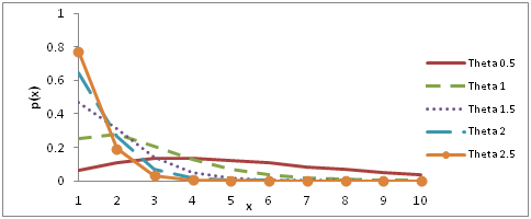
Behavior of the pmf of SBDLD (2.1) for varying values of the parameter has been drawn in Figure 1. It would be recalled that the pmf of size-biased Poisson-Lindley distribution (SBPLD) having parameter given by
(2.5)
Has been introduced by Ghitany & Mutairi13 which is a size-biased version of Poisson-Lindley distribution (PLD) introduced by Sankaran,11 Ghitany & Mutairi13 have discussed its various mathematical and statistical properties, estimation of the parameter using maximum likelihood estimation and the method of moments, and goodness of fit Shanker et al.14 has critical study on the applications of SBPLD for modeling data on thunderstorms and found that SBPLD is a better model for thunderstorms than size-biased Poisson distribution (SBPD).

Figure 1 Behavior of pmf of SBDLD for varying values of the parameter
.
Moments
The probability generating function (G(t)) and the moment generating function (M(t)) of SBDLD can be obtained as
, (3.1)
and
. (3.2)
It can be easily verified that the function in (3.2) is infinitely differentiable with respect to , since it involves exponential terms of its argument. This means that all moments about origin of SBDLD can be obtained. The rth moment about origin of SBDLD (2.1) can be obtained as
Taking and simplifying the complicated and tedious algebraic expression, the first four raw moments (moments about the origin) of the SBDLD (2.1) can be obtained as
Now, using the relationship between central moments (moments about mean) and the raw moments, the central moments of the SBDLD (2.1) can be obtained as
The coefficient of variation , coefficient of Skewness , coefficient of Kurtosis and index of dispersion of the SBDLD (2.1) are thus given as
It can be easily verified that SBDLD is over-dispersed , equi-dispersed and under-dispersed for . It should be noted that SBPLD is over-dispersed , equi-dispersed and under-dispersed for . The behavior of mean, variance, C.V, skewness, kurtosis and index of dispersion for varying values of parameter has been shown numerically in Table 1.
Theta |
Mean |
|
Variance |
CV |
Skewness |
Kurtosis |
Index of dispersion |
0.25 |
47.7508 |
|
11.5624 |
0.5976 |
1.1637 |
5.0209 |
4.1298 |
0.50 |
11.7531 |
|
5.6245 |
0.6095 |
1.1910 |
5.0851 |
2.0896 |
0.75 |
5.0902 |
|
3.6858 |
0.6121 |
1.2368 |
5.1965 |
1.3810 |
1.00 |
2.7620 |
|
2.7459 |
0.6052 |
1.3021 |
5.3621 |
1.0059 |
1.25 |
1.6884 |
|
2.2047 |
0.5894 |
1.3877 |
5.5923 |
0.7658 |
1.50 |
1.1091 |
|
1.8617 |
0.5657 |
1.4950 |
5.9016 |
0.5958 |
1.75 |
0.7637 |
|
1.6310 |
0.5358 |
1.6257 |
6.3095 |
0.4682 |
2.00 |
0.5430 |
|
1.4696 |
0.5015 |
1.7818 |
6.8415 |
0.3695 |
2.25 |
0.3951 |
|
1.3535 |
0.4644 |
1.9658 |
7.5310 |
0.2919 |
2.50 |
0.2923 |
|
1.2683 |
0.4263 |
2.1806 |
8.4215 |
0.2304 |
2.75 |
0.2189 |
|
1.2049 |
0.3883 |
2.4294 |
9.5689 |
0.1817 |
3.00 |
0.1654 |
|
1.1572 |
0.3515 |
2.7163 |
11.0451 |
0.1430 |
Table 1 Values of coefficient of variation, skewness, kurtosis, index of dispersion, mean and variance of SBDLD for different values of parameter
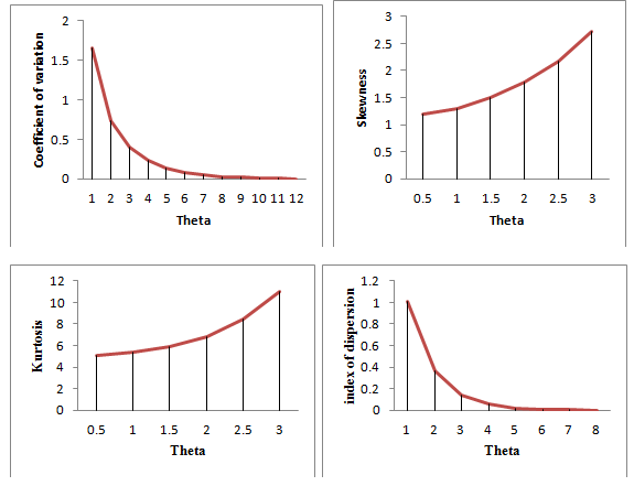
The behavior of coefficient of variation , coefficient of Skewness , coefficient of Kurtosis and index of dispersion
of the SBDLD are shown in Figure 2. From Figure 2, it is obvious that C.V and index of dispersion are monotonically decreasing whereas coefficient of skewness and coefficient of kurtosis are monotonically increasing for increasing values of the parameter .

Figure 2 Behavior of C.V, coefficient of Skewness, coefficient of Kurtosis and index of dispersion of the SBDLD for varying values of the parameter
.
The behavior of mean and variance for varying values of parameter has been shown in Figure 3.

Figure 3 Behavior of Mean and Variance of the SBDLD for varying values of the parameter
.
Estimation of parameter
Method of Moment Estimate (MOME)
Equating the population mean to the corresponding sample mean, the method of moment estimate (MOME)
of of SBDLD (2.1) is given by
,
Where is the sample mean.
Maximum Likelihood Estimate (MLE)
Let
be a random sample of size
from the SBDLD (2.1) and let be the observed frequency in the sample corresponding to such that , where is the largest observed value having non-zero frequency. The likelihood function of the SBDLD (2.1) is given by
The log likelihood function can be obtained as
The first derivative of the log likelihood function is thus given by
,
Where is the sample mean. The maximum likelihood estimate (MLE), of of SBDLD (2.1) is the solution of the equation and is given by
Thus, like DLD, both MOME and MLE give the same estimate of the parameter in case of SBDLD.
Goodness of fit
We know that size-biased distributions are useful for modeling data relating to situation when organisms occur in groups and the group size influence the probability of detection. In this section, the goodness of fit of SBDLD has been discussed with data relating to the size distribution of freely -forming small groups at various public places, reported by James15 and Coleman & James.16 The expected frequency by size-biased Poisson distribution (SBPD) and size-biased Poisson-Lindley distribution (SBPLD) have also been presented for ready comparison with SBDLD. Note that the goodness of fit of SBDLD, SBPD and SBPLD is based on the maximum likelihood estimates of the parameter.
Based on the values of chi-square () and p-value, it is obvious that SBDLD gives much closer fit than SBPD and SBPLD in the Tables 2-4 while in Table 5, SBPLD gives much closer fit than both SBPD and SBDLD. Thus, SBDLD can be considered an important distribution for modeling the distribution of freely-forming small group size at various public places.
Group Size |
Observed Frequency |
Expected Frequency |
SBPD |
SBPLD |
SBDLD |
1
2
3
4
5
6 |
1486
694
195
37
10
1 |
1452.4
743.3
190.2
32.4
4.1
0.6 |
1532.5
630.6
191.9
51.3
12.8
3.9 |
1486.4
693.0
193.9
41.0
7.3
1.4 |
Total |
2423 |
2423.0 |
2423.0 |
2423 |
ML estimate |
|
|
|
|
|
|
7.370 |
1.760 |
1.007 |
d.f. |
|
2 |
3 |
3 |
p-value |
|
0.0251 |
0.0030 |
0.9088 |
Table 2 Pedestrians-eugene, spring, morning
Group Size |
Observed Frequency |
Expected Frequency |
SBPD |
SBPLD |
SBDLD |
1
2
3
4
5 |
316
141
44
5
4 |
306.3
156.2
39.8
6.8
0.9 |
323.0
132.5
40.2
10.7
3.6 |
313.4
145.6
40.6
8.6
1.8 |
Total |
510 |
510.0 |
510.0 |
510.0 |
ML estimate |
|
|
|
|
|
|
2.463 |
3.020 |
0.640 |
d.f. |
|
2 |
2 |
2 |
p-value |
|
0.4818 |
0.3884 |
0.8872 |
Table 3 Shopping groups–eugene, spring, department store and public market
Group Size |
Observed Frequency |
Expected Frequency |
SBPD |
SBPLD |
SBDLD |
1
2
3
4
5
6 |
305
144
50
5
2
1 |
296.5
159.0
42.6
7.6
1.0
0.3 |
314.4
134.4
42.5
11.8
3.1
0.8 |
304.1
148.0
43.2
9.5
1.8
0.4 |
Total |
507 |
507.0 |
507.0 |
507 |
ML estimate |
|
|
|
|
|
|
3.035 |
6.415 |
2.351 |
d.f. |
|
2 |
2 |
2 |
p-value |
|
0.2190 |
0.0400 |
0.5028 |
Table 4 Play groups–eugene, spring, public playground D
Number times hares caught |
Observed Frequency |
Expected Frequency |
SBPD |
SBPLD |
SBDLD |
1
2
3
4
5 |
306
132
47
10
2 |
292.2
155.2
41.2
7.3
1.1 |
309.4
131.2
41.1
11.3
4.0 |
299.5
144.5
41.8
9.1
2.1 |
Total |
497 |
497.0 |
497.0 |
497 |
ML estimate |
|
|
|
|
|
|
6.479 |
0.932 |
1.926 |
d.f. |
|
2 |
2 |
2 |
p-value |
|
0.0390 |
0.6281 |
0.5878 |
Table 5 Play groups–eugene, spring, public playground A
Concluding remarks
In the present paper size-biased discrete Lindley distribution (SBDLD), a simple size-biased version of the discrete Lindley distribution (DLD) of Berhane & Shanker1 has been proposed and studied. Its raw moments and central moments have been obtained and hence expressions for coefficient of variation, skewness, kurtosis and index of dispersion have been presented and their behaviors have been discussed graphically. The estimation of its parameter has been discussed using the method of moments and the method of maximum likelihood. The goodness of fit of the SBDLD has been discussed with four examples of observed real datasets relating to freely-forming small group size at public places over SBPD and SBPLD and the fit given by SBDLD gives quite satisfactory fit. Therefore, SBDLD can be considered an important distribution for modeling count data relating to freely-forming small group size at public places.
Acknowledgement
Conflict of interest
The author declares there is no conflict of interest.
References
- Berhane A, Shanker R. A discrete Lindley distribution with applications in Biological sciences. Biometrics & Biostatistics International Journal. 2018;7(2):1–5.
- Fisher RA. The effects of methods of ascertainment upon the estimation of frequencies. Annals of Eugenics. 1934;6(1):13–25.
- Rao CR. On discrete distributions arising out of methods of ascertainment. In: Patil GP, editor. Classical and Contagious Discrete Distributions. India: Statistical Publishing Society; 1965:320–332.
- Patil GP, Ord JK. On size–biased sampling and related form–invariant weighted distributions. Sankhyā: The Indian Journal of Statistics, Series B. 1976;38(1):48–61.
- Patil GP, Rao CR. The Weighted distributions: A survey and their applications. In: Krishnaiah PR, editor. Applications of Statistics. Netherlands: North Holland Publications; 1977:383–405.
- Patil GP, Rao CR. Weighted distributions and size–biased sampling with applications to wild-life populations and human families. Biometrics. 1978;34:179–189
- Patil GP. Studies in statistical ecology involving weighted distributions. In: Ghosh JK, Roy J, editors. Applications and New Directions. Proceeding of Indian Statistical Institute. Golden Jubliee, India: Statistical Publishing society; 1981:478–503.
- Lindley DV. Fiducial distributions and Bayes theorem. Journal of the Royal Statistical Society. 1958;20(1):102–107.
- Ghitany ME, Atieh B, Nadarajah S. Lindley distribution and its Application. Mathematics Computing and Simulation. 2008;78(4):493–506.
- Shanker R, Hagos F, Sujatha S. On modeling of lifetimes data using exponential and Lindley distributions. Biometrics & Biostatistics International Journal. (2015);2(5):1– 9.
- Sankaran M. The discrete Poisson–Lindley distribution. Biometrics. 1970;26(1):145–149.
- Barlow RE, Proschan F. Statistical Theory of Reliability and Life Testing. USA: Silver Spring; 1981.
- Ghitany ME, Al–Mutairi DK. Size–biased Poisson–Lindley distribution and Its Applications. Metron–International Journal of Statistics. 2008;16(3):299–311.
- Shanker R, Hagos F, Abrehe Y. On Size–Biased Poisson–Lindley Distribution and Its Applications to Model Thunderstorms. American Journal of Mathematics and Statistics. 2015;5(6):354–360.
- James J. The distribution of freely–forming small group size. American sociological Review. 1953;18:569–570.
- Coleman JS, James J. The equilibrium size distribution of freely–forming groups. Sociometry. 1961;24(1):36–45.

©2018 Sium, et al. This is an open access article distributed under the terms of the,
which
permits unrestricted use, distribution, and build upon your work non-commercially.


