In many applications related to time to event data, especially in the medical field, it is common the presence of a fraction of individuals not expecting to experience the event of interest, these individuals immune to the event or cured for the disease during the study are known as long–term survivors. To estimate survival and hazard curves, in this situation, it is common the use of Weibull cure rate model due to its great flexibility and simplicity. In this paper, we present the estimation of survival and hazard curves using a extension of Mirra model using the classical cure rate approach and applying it to gastric and breast cancer data. The inferences of interest were obtained using a Bayesian approach and the results achieved from this study showed that the Mirra model has a good fit and could be an useful alternative for estimation and shape prediction of survival and hazard curves for long–term survivors, especially for cancer data. The results could be extended using regression approach in order to identify risk factor that affects the survival probability.

Keywords: bayesian approach, breast cancer, cure rate models, gastric cancer, survival analysis

In many health studies, powerful tools for the statistical analysis are the survival analysis techniques that could be useful, for example, to identify risk factors or treatments that influences the survival or cure probability of a certain disease. In general, survival analysis consists in a set of techniques and statistical models commonly used when the random variable of interest is the time until the occurrence of a specific event, such as the time until the occurrence of a disease or the time until the patient’s death. A concept that differs survival analysis from others statistical analysis is the presence of censored data that occur when we have partial individual information about the time of occurrence of the variable of interest, however we do not know the exact time of occurrence of the event, that is, the real time of occurrence may exceed the observed time. The censored data can occur for a variety of reasons as the loss of monitoring of the patient over time and the non–occurrence of the event of interest until the end of the experiment. According to Colosimo and Giolo¹ there are two reasons that justify the use of censored data in statistical analysis: (I) although these observations are not complete, they provide information about the patient’s lifetime and (II) the omission of the observations censored can lead to the calculation of biased estimates.

In survival analysis, usual parametric and non–parametric tools are widely used for analyzing data from time to event data. These tools are useful when some observations are censored and the event of interest was not seen in all patients during the follow–up period. The most used procedures include the mortality table, the Kaplan–Meier estimator for the survival function, the Cox proportional hazards model and parametric survival models. Parametric models are more flexible than Cox proportional hazards model, especially when there is no proportionality of risks between groups and are based mainly on two important functions, the survival function and the hazard function. These techniques are described in several textbooks as Kalbeisch and Prentice,² Klein and Moeschberger³ and Kleinbaum and Klein.⁴

Let a non–negative random variable T related to the failure time, then the survival function is defined as the probability that an observation will not fail until a certain time t, that is, the probability that an observation will survive time t. In probabilistic terms,

$S(t)=P(T\ge t)$

On other hand, the hazard function $\lambda (t)$ represents the instantaneous failure rate at time  $t$ conditional on survival time $t$ and is very useful to describe the distribution of patient’s lifetime. In probabilistic terms,

$\lambda (t)=\underset{\Delta t\to 0}{\text{lim}}\frac{P(t\le T<t+\text{Δ}t|T\ge t)}{\text{Δ}t}.$

Nonetheless, a common situation in many lifetime studies, particularly in cancer research, occurs when it is expected that a fraction of individuals will not experience the event of interest, this fraction of individuals often are immune or are cured. The presence of immune or cured individuals in a data set is usually suggested by a Kaplan–Meier plot of the survival function, which shows a long and stable plateau, with several censored date at the extreme right of the plot.^5–8 However, an efficient and commonly applied technique is to consider a mixture of two populations, one susceptible to the event of interest adopting a base probability distribution to model the survival time of susceptible patients, and one of the most common distributions as, for example, the Weibull distribution^9–11 for the non–susceptible population.

According to Hjorth,¹² one or two parameters distributions have some important limitations such as the inability to model data that presents a bathtub risk function, for example. However, the most flexible distributions and with the largest number of parameters, may have inaccurate estimates, when there is a small sample size. In this way, this paper present a mixture cure rate model based on the Mirra distribution¹³ to estimate survival and hazard curves. The choice of Mirra distribution is justified due it number of parameters (two–parameters) and the bathtub shapes for the hazard function. Two dataset sets are considered to illustrate the proposed methodology. The first, related to gastric cancer, presents the bathtub shape for the empirical hazard function; and the second, related to breast cancer, presents a decreasing shape for the empirical hazard function.

The paper is organized as follows: in Section 2, it is presented the mixture Mirra cure rate model as its likelihood function. A brief description of the Bayesian approach and some discrimination criteria are also presented in Section 2. Section 3 presents the statistical analysis based on mixture Mirra cure rate model for two cancer data: gastric and breast cancer. The estimation of the survival and hazard curves are also presented in Section 3. Finally, Section 4 close the paper with some concluding remarks.

The mirra distribution

A first approach of the Mirra distribution (TPM) was introduced in the literature by Subhradev Sen.¹³ These authors studied most of it properties and illustrate how the Mirra distribution was synthesized as a special finite mixture of exponential and gamma distributions. In this way, let $T$ be a continuous random variable following Mirra distribution with parameters $\alpha$ and $\theta$ . The probability density function (pdf) and survival function (sf) of the random variable $T$ is given, respectively, by,

$f\left(t\right)=\frac{{\theta }^3}{{\theta }^2+\alpha }\left(1+\frac{1}{2} \alpha t^2\right)e^{-\theta t},$ (3)

 and,

$S\left(t\right)=\frac{{\theta }^2}{{\theta }^2+\alpha }\left(1+\frac{1}{{\theta }^2} \alpha +\frac{1}{\theta } \alpha t+\frac{1}{2} \alpha t^2\right)e^{-\theta t}.$ (4)

 where $t>0$ and $\alpha ,\theta >0$ . Thus, the hazard function (hf) is represented by,

$\lambda \left(t\right)=\frac{\theta \left(1+\frac{1}{2} \alpha t^2\right)}{\left(1+\frac{1}{{\theta }^2} \alpha +\frac{1}{\theta } \alpha t+\frac{1}{2} \alpha t^2\right)}.$ (5)

As noted by Subhradev Sen¹³ the hf of this distribution has the shape of a bathtub, decreasing to $t<\sqrt{\frac{2}{\alpha }}$ and increasing to $t>\sqrt{\frac{2}{\alpha }}$ . Moreover, these authors also showed that the hf is limited with the following limits,

$\frac{2{\theta }^3}{\alpha +2{\theta }^2+\theta \sqrt{2\alpha }}<\lambda (t)<\theta .$ (6)

In Figure 1, it is illustrated the shape of pdf, sf and hf. From those plots, it is possible to see the bathtub shape for the hf (green line). Also, for example, assuming $\alpha =5,\theta =2$ (green line), we have that the limits of the hf are given by $0.828<\lambda (t)<2.000$ .

Figure 1 Behavior of the pdf (left panel), sf (middle panel) and hf (right-panel) for TPM distribution assuming arbitrary values for the parameters $\alpha$  and $\theta$ .

A great advantage for the use of TPM distribution is that the special cases maintain the bathtub shape for the hf. These cases are described by, 

1. When we consider $\alpha =1$ , we get the Mirra–silence distribution (MSI), with probability density function and survival function respectively given by

$f\left(t\right)=\frac{{\theta }^3}{1+{\theta }^2}\left(1+\frac{1}{2} t^2\right)e^{-\theta t} \text{and} S\left(t\right)=\frac{{\theta }^2}{1+{\theta }^2}\left(1+\frac{1}{{\theta }^2}+\frac{1}{\theta } t+\frac{1}{2} t^2\right)e^{-\theta t}$ (7)

2. In case of $\theta =1$ , is obtained the Mirra–surrender distribution (MSII), with probability density function and survival function respectively given by

$f\left(t\right)=\frac{1}{1+\alpha }\left(1+\frac{1}{2} \alpha t^2\right)e^{-t} \text{and} S\left(t\right)=\frac{1}{1+\alpha }\left(1+\frac{1}{{\theta }^2} \alpha +\frac{1}{\theta } \alpha t+\frac{1}{2} \alpha t^2\right)e^{-\theta t}$ (8)

3. If we consider $\alpha =\theta =\beta$ , we have in this case the the xgamma distribution (XG), proposed by Sen et al.,¹⁴ with probability density function and survival function respectively given by

$f\left(t\right)=\frac{{\beta }^2}{1+\beta }\left(1+\frac{1}{2} \beta t^2\right)e^{-\beta t} \text{and} S\left(t\right)=\frac{\beta }{1+\beta }\left(1+t+\frac{1}{\beta }+\frac{1}{2} \beta t^2\right)e^{-\beta t}.$ (9)

Mixture mirra cure rate model

Let us denote by $T$ the event of interest. Following Maller and Zhou,¹⁵ the standard cure rate model (or mixture cure rate model) assuming that the probability of the time–to–event to be greater than a specified time $t$ is given by the survival function,

$S(t)=\rho +(1-\rho )S_0(t)$ (10)

where $\rho \in (0,1)$ is the mixing parameter which represents the proportion of “long–term survivors”, “non–susceptible” or “cured patients”, and $S_0(t)$ denotes a proper survival function for the non–cured or susceptible group in the population. Observe that if $t\to \infty$ , then $S(t)\to \rho$ , that is, the survival function has an asymptote at the cure rate $\rho$ . The probability density and the hazard functions corresponding to (10) are given, respectively, by,

$f(t)=(1-\rho )f_0(t)$ (11)

 and,

$\lambda (t)=\frac{(1-\rho )f_0(t)}{\rho +(1-\rho )S_0(t)}$ (12)

Now, assuming TPM distribution by the Equation (4) as the baseline sf for the susceptible individuals in the Equation (10), we get the mixture TPM cure rate model with sf and pdf given, respectively, by

$S(t)=\rho +\frac{(1-\rho ){\theta }^2}{{\theta }^2+\alpha }\left(1+\frac{1}{{\theta }^2} \alpha +\frac{1}{\theta } \alpha t+\frac{1}{2} \alpha t^2\right)e^{-\theta t},$ (13)

 and,

$f(t)=\frac{(1-\rho ){\theta }^3}{{\theta }^2+\alpha }\left(1+\frac{1}{2} \alpha t^2\right)e^{-\theta t}.$ (14)

The likelihood function

Let $T$ be a positive random variable denoting the survival time of a patient and $U$ another positive random variable denoting the censoring or dropout time of the patient. Also define an indicator variable (binary variable) of censoring for the $i{}^{th}$ patient defined by $d_i=1$ , for $T=t_i$ and $U\ge t_i$ and $d_i=0$ for $T>t_i$ and $U=t_i$ , where $t_i=\text{min}(T_i,U_i)$ . For the $i{}^{th}$ patient, $i=1,2,\dots ,n$ , the contribution for the log–likelihood function is given by,

$\ell ={\displaystyle {\sum }_{i=1}^n{d}_i}\log \left[f(t_i)\right]+{\displaystyle {\sum }_{i=1}^n(1-d_i)\text{log}\left[S(t_i)\right]}$ (15)

where $f(t_i)$ and $S(t_i)$ denotes, respectively, the pdf and sf associated to the $i{}^{th}$ patient. Now, assuming the mixture TPM cure rate model with a parameter vector $\psi =(\alpha ,\theta ,\rho )$ , we have, for the $i{}^{th}$ patient, $i=1,2,\dots ,n$ , the contribution for the log–likelihood function is given by,

$\begin{array}{l}\ell (\psi )=\text{l}n\left(1-\rho \right){\displaystyle {\sum }_{i=1}^n{d}_i}+\text{l}n\left({\theta }^3\right){\displaystyle {\sum }_{i=1}^n{d}_i}-ln\left({\theta }^2+\alpha \right){\displaystyle {\sum }_{i=1}^n{d}_i}+{\displaystyle {\sum }_{i=1}^n{d}_i}\text{ln}\left(1+\frac{1}{2}{\alpha }_i^2\right)\\ +\theta {\displaystyle {\sum }_{i=1}^n{d}_i}{t}_i+{\displaystyle {\sum }_{i=1}^n\left(1-d_i\right)}\left[\rho +\frac{\left(1-\rho \right){\theta }^2}{{\theta }^2+\alpha }\left(1+\frac{1}{{\theta }^2}\alpha +\frac{1}{\theta }\alpha t_i+\frac{1}{2}\alpha t_i^2\right)e^{-\theta t_i}\right]\end{array}$ (16)

Bayesian analysis

In general, the statistical inference is the process of data analysis to deduce properties of a population from a sampled data of that population. According to Ibrahim et al.,¹⁶ the Bayesian paradigm is based on specifying a probability model for the observed data $D$ , given a vector of unknown parameters $\theta$ and provides a rational method for updating the new information using the Bayes’ rule and prior distributions for the uncertainty about $\theta$ . That is, the Bayesian paradigm is the process of fitting a probability model to a set of data and summarizing the result by a probability distribution, called posterior distribution, on the parameters of the model and on unobserved quantities such as predictions for new observations. In this way, assuming the proposed mixture TPM cure rate model, we simulate samples from the joint posterior distribution using the MCMC (Markov Chain Monte Carlo) algorithm implemented in the OpenBUGS software, a free version of WinBUGS software,¹⁷ by the package “BRugs"¹⁸ from R software.¹⁹

For the Bayesian analysis, as prior distributions, we adopted approximately non–informative gamma prior distributions, $G(a,b)$ , for the parameters $\alpha ,\theta$ , where $a$ and $b$ are known hyperparameters, and $G(a,b)$ denotes a gamma distribution with mean $a/b$ and variance $a/b^2$ . Moreover, for the parameter $\rho$ we assume a prior beta distribution $\rho \sim Beta(1,1)$ since $\rho \in (0,1)$ . The posterior summaries of interest are computed adopting a burn–in sample of size 50,000 to eliminate the effect of the initial values and a final Gibbs sample of size 4,000 taking every 50th sample from 250,000 simulated Gibbs samples. Also, the  highest probability density (95% HPD)²⁰ interval was considered for the Bayesian estimates. The convergence procedures based on traceplots were verified using the “coda"²¹ package from R software.

To discriminate between models in the statistical analysis, two criteria are considered here: the deviance information criterion (DIC) and the extended Bayesian information criteria (EBIC). The DIC is a criterion specially useful for selection models under the Bayesian approach where samples of the posterior distribution for the parameters of the model are obtained using MCMC methods. It is similar to AIC criteria with two changes: replace the maximum likelihood estimate $\stackrel{⌢}{\theta }$ with posterior mean ${\stackrel{⌢}{\theta }}_{Bayes}=\mathbb{E}\mathbb{A}\theta |\text{y}\mathbb{A}$ and replace $k$ with a data–based bias correction. The new measure of predictive accuracy, according to Spiegelhalter et al.,²² is,

${\stackrel{⌢}{elpd}}_{\text{DIC}}=\text{log}p(\text{y}|{\stackrel{⌢}{\theta }}_{Bayes})-p_{\text{DIC}},$ (17)

where P_DIC is the effective number of parameters, defined as,

$p_{\text{DIC}}=2\left(\text{log}p(\text{y}|{\stackrel{⌢}{\theta }}_{Bayes}-{\mathbb{E}}_{post}(\text{log}p(\text{y}|\theta )\right),$ (18)

 where the expectation in the second term is an average of $\theta$ over its posterior distribution. The posterior mean of $\theta$ will produce the maximum log predictive density when it happens to be the same as the mode, and negative $p_{\text{DIC}}$ can be produced if posterior mean is far from the mode (Spiegelhalter et al.,²²). Finally, the actual quantity called DIC is defined in terms of the deviance rather than the log predictive density. Thus,

$\text{DIC}=-2\text{log}p(\text{y}|{\stackrel{⌢}{\theta }}_{Bayes})+2p_{\text{DIC}}$ (19)

 Smaller values of DIC indicate better models with a difference at least 5 by each model in DIC values.²³ Note that these values could be negative. On other hand, the extended Bayesian information criteria (EBIC), proposed by Chen and Chen²⁴, is given

$\text{EBIC}=\overline{D(\theta )}+k\text{ln}(n),$ (20)

where $\overline{D}=E[D(\theta )]$ , is the posterior mean of the deviance, $k$ is the number of model parameters and $n$ is the sample size. The EBIC has the advantage of penalizing the model by the number of parameters.

In this section, we present the usefulness of the proposed mixture TPM cure rate to estimate survival and hazard curves in cancer research under a Bayesian approach. For the hyperparameters of the gamma prior distributions, we adopted a=b=1. The results showed that the mixture TPM cure rate model is great do describe the survival probabilities as well the bathtub shape from the empirical hazard function of the data. The model also shows good lengths (small values for the difference between lower and upper bound) for the 95% HPD interval which is a indication of good fit.

Gastric cancer data

The gastric cancer is one of the leading causes of cancer–related death. Several studies are carried out to advance our understanding of the biologic behavior of gastric cancer and improve surgical management and outcome.²⁵ To illustrate the usefulness of the proposed methodology, we considered a dataset related to the times until death in months since surgery of 201 patients of different clinical stages, obtained by Jacome et al.²⁶ who carried out a retrospective study in patients with gastric adenocarcinoma who underwent curative resection with D2 lymphadenectomy in the Barretos Cancer Hospital (Brazil) between January 2002 and December 2007. For more details of the dataset, the reader should consult Martinez et al.²⁷ The posterior summaries of interest for parameters of the mixture TPM cure rate model are presented in Table 1 and the fit of mixture TPM cure rate model was compared to the fit of the mixture MSI, MSII and XG cure rate models (the special cases of the TPM model). By the both discrimination criteria, it could be concluded that the mixture TPM cure rate model is the best model fitted for the dataset.

In Figure 2, it is presented the estimated survival (left panel) and hazard (right panel) curves for each model considered in the analysis. From the Kaplan–Meier curve for the empirical survival function, it could be seen a plateau close to the value 0.5 which was great estimated by all models. However, assuming the MSII model, the survival curve is poorly estimated. On other hand, for the hazard curve, only the TPM model has a good fit to capture the bathtub shape from the empirical hazard function (obtained using the package “bshazard").²⁸ The other models present some values out of the confidence bounds from the empirical hazard function. Finally, in 3, it is present the probability plots for each model where it could be seen that the TPM model has a good fit for the gastric cancer data.

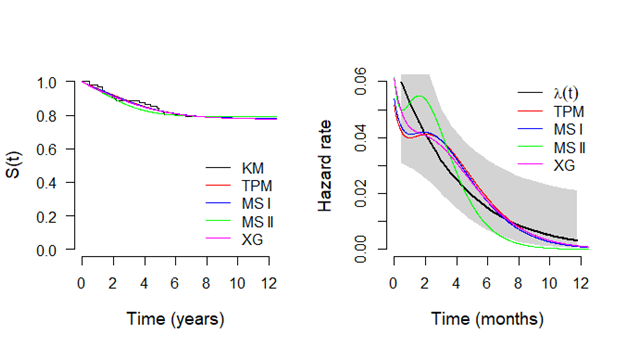
Figure 2 Plots of the survival functions estimated by Kaplan-Meier method and from the mixture cure fraction model based on TPM distribution and special cases (left panel) and respective hazard functions (right panel), considering gastric cancer data

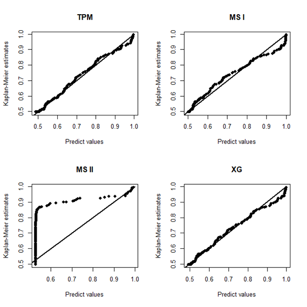
Figure 3 Plots of the Kaplan-Meier estimates for the survival function versus the respective predict values obtained from the mixture models based on TPM distribution and special cases, considering gastric cancer data.

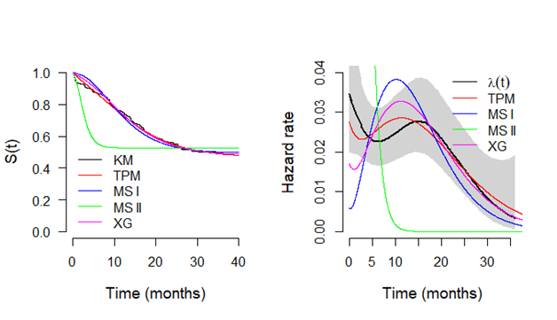
Figure 4 Plots of the survival functions estimated by Kaplan-Meier method and from the models based on TPM distribution and special cases (left panel) and respective hazard functions (right panel), considering breast cancer data.

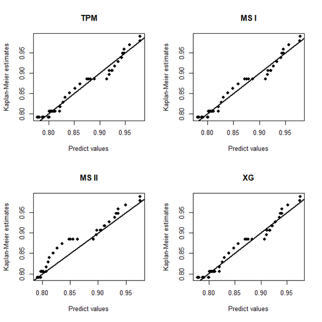
Figure 5 Plots of the Kaplan-Meier estimates for the survival function versus the respective predict values obtained from the mixture models based on TPM distribution and special cases, considering breast cancer data.

In conclusion, the proposed mixture TPM cure rate model is adequate to model the lifetime of the patients with gastric cancer and the shape of the hazard function which could be useful in medical studies that the main interest is how to describe or predict hazard curves. In addition, comparing with the results obtained by Martinez et al.,²⁷ no significant differences were found in the estimated cure fraction, however, it is worth mentioning that the model proposed in this manuscript has simpler equation, less number of parameters and flexibility of the hazard function which could be more useful that the model adopted in Martinez et al.,²⁷ especially for the bathtub shape of hazard function of the data.

Breast Cancer Data

According Bray et al.²⁹ the breast cancer is the most common cancer in women worldwide, other than non–melanoma skin cancer. However, with the advancement of treatments the proportion of cure increased considerably.³⁰ To illustrate the usefulness of the proposed methodology, we considered now a dataset related related to a cohort study where 97 patients underwent surgical treatment for breast cancer followed up for a period ranging from the year 2000 to 2011. More details of this study can be found in Shigemizu et al.,³¹ For more details of the dataset, the reader should consult Shigemizu et al.³¹ As lifetime, it was considered the overall survival time (OS), that is, the lifetime after the diagnosis or started treatment. The posterior summaries of interest for parameters of the mixture TPM cure rate model are presented in Table 2. By the both discrimination criteria, it could be concluded that there is no significant difference for DIC values among the considered models and, by the EBIC criteria, the mixture TPM cure model may not be the most suitable for this data. This fact occurs due to the penalty that the EBIC put on the number of parameters of the model.

In Figure 2, it is presented the estimated survival (left panel) and hazard (right panel) curves for each model considered in the analysis. From the Kaplan–Meier curve for the empirical survival function, it could be seen a plateau close to the value 0.8 which was great estimated by all models. For the hazard curve, all the models have a good fit to capture the decreasing shape from the empirical hazard function. Finally, in 3, it is present the probability plots for each model where it could be seen that the probability plots are basically identical for each model and implying in a reasonable fit for each model assuming the breast cancer data.

In this study, it was introduced a new univariate cure rate model using the mixture approach and the TPM distribution introduced by Subhradev Sen¹³ in order to estimate the survival and hazard curves in medical application related to cancer data. The main advantage of the proposed model is the number of parameters and the incorporation of the bathtub shape from hazard function that is common in cancer data.

In the applications considered here, we can conclude that the proposed cure rate model could be really useful. For example, in the application with gastric cancer, the proposed mixture TPM cure model showed a good fit and was the only one that captured the bathtub shape from the empirical hazard function within the confidence bounds. On other hand, despite the good fit from all considered models in the breast cancer application, the proposed model also capture the shape of the empirical hazard function within confidence bounds. Now, assuming the survival curves, in both applications, the proposed model captured the cure rate as well the entire survival curve, being great to predict survival probabilities.

In conclusion, the results emerging from this study reinforce the fact that the search of appropriate lifetime distribution could be extremely difficult, especially, depending on the shape of the empirical hazard function of the data. However, the proposed methodology could be very useful in the medical data analysis where the interest is the estimation of the fraction of patients in the studied population who never experience the event of interest. The results could be also extended to other cross–over trials in clinical research; reliability analysis in engineering; risk analysis in economics; among many others areas.

The authors declare that they have no conflicts of interest.

None.

1. Colosimo EA, Giolo SR. Análise de Sobrevivência Aplicada. Edgard Blucher, Sao Paulo.
2. Kalbeisch JD, Prentice RL. The statistical analysis of failure time data. John Wiley & Sons, 2 edition.
3. Klein JP, Moeschberger ML. Survival analysis: techniques for censored and truncated data. Springer Science & Business Media. 2003.
4. Kleinbaum DG, Klein M. Survival analysis. volume 3. Springer. 2010.
5. Corbière F, Commenges D, Taylor JM, et al. A penalized likelihood approach for mixture cure models. Statistics in medicine. 2009;28(3):510–524.
6. Lambert PC, Thompson JR, Weston CL, et al. Estimating and modeling the cure fraction in population–based cancer survival analysis. Biostatistics. 2006;8(3):576–594.
7. Chen MH, Ibrahim JG, Sinha D. et al. Bayesian inference for multivariate survival data with a cure fraction. Journal of Multivariate Analysis. 2001;80(1):101–126.
8. Wienke A. Frailty models in survival analysis. CRC press. 2010.
9. Weibull W. A statistical distribution function of wide applicability. Journal of Applied Mechanics. 1951;18(3):293–297.
10. Rinne H. The Weibull distribution: a handbook. CRC press. 2008.
11. McCool JI. Using the Weibull distribution: reliability, modeling, and inference, volume 950. John Wiley & Sons. 2012.
12. Hjorth U. A reliability distribution with increasing, decreasing, constant and bathtubshaped failure rates. Technometrics. 1980;22(1):99–107.
13. Sen S, Ghosh SK, Al–Mofleh H. The mirra distribution for modeling time–to event data set. In International Conference on Strategic Management, Decision Theory and Data Science.
14. Sen S, Maiti SS, Chandra N. The xgamma distribution: statistical properties and application. Journal of Modern Applied Statistical Methods. 2016;15(1):38.
15. Maller RA, Zhou X. Survival analysis with long–term survivors. Wiley New York. 1996.
16. Ibrahim JG, Chen MH, Sinha D. Bayesian survival analysis. Wiley Online Library. 2005.
17. Lunn DJ, Thomas A, Best N, et al. Winbugs–a bayesian modeling framework: concepts, structure, and extensibility. Statistics and computing. 2000;10(4):325–337.
18. Thomas A, O'Hara B, Ligges U, et al. Making bugs open. R News. 2006;6(1):12–17.
19. R Core Team. R: A Language and Environment for Statistical Computing. R Foundation for Statistical Computing, Vienna, Austria. 2020.
20. Chen MH, Shao QM. Monte carlo estimation of bayesian credible and hpd intervals. Journal of Computational and Graphical Statistics. 1999;8(1):69–92.
21. Plummer M, Best N, Cowles K, et al. Coda: Convergence diagnosis and output analysis for mcmc. R News. 2006;6(1):7–11.
22. Spiegelhalter DJ, Best NG, Carlin BP, et al. Bayesianmeasures of model complexity and fit. Journal of the Royal Statistical Society: Series B(Statistical Methodology). 2002;64(4):583–639.
23. Box GE, Tiao GC. Bayesian inference in statistical analysis. volume 40. John Wiley & Sons. 2011.
24. Chen J, Chen Z. Extended bayesian information criteria for model selection with large model spaces. Biometrika. 2008;95(3):759–771.
25. Dicken BJ, Bigam DL, Cass C, et al. Gastric adenocarcinoma: review and considerations for future directions. Ann Surg. 2005;241(1):27.
26. Jácome AA, Wohnrath DR, Neto CS, et al. Effect of adjuvant chemoradiotherapy on overall survival of gastric cancer patients submitted to d2 lymphadenectomy. Gastric Cancer. 2013;16(2):233–238.
27. Martinez EZ, Achcar JA, Jácome, AA, et al. Mixture and nonmixture cure fraction models based on the generalized modi_ed weibull distribution with an application to gastric cancer data. Computer methods and programs in biomedicine. 2013;112(3):343–355.
28. Paola Rebora AS, Reilly M. bshazard: Nonparametric smoothing of the hazard function. R package version 1.1. 2018.
29. Bray F, Ferlay J, Soerjomataram I, et al. Global cancer statistics 2018: GLOBOCAN estimates of incidence and mortality worldwide for 36 cancers in 185 countries. A cancer for journal clinicians. 68(6):394–424.
30. Waks AG, Winer EP. Breast cancer treatment: a review. JAMA. 2019;321(3):288–300.
31. Shigemizu D, Iwase T, Yoshimoto M, et al. The prediction models for postoperative overall survival and disease–free survival in patients with breast cancer. Cancer Med. 2017;6(7):1627–1638.