Many studies consider clustered data that are measured on participants over time. Examples include the collection of repeated systolic and diastolic blood pressure on patients, or of serial assessment of Vitamin D sufficiency (yes/no) on people living within defined geographic regions. This manuscript describes our user-written SAS macro, %qlsmultcorr, which can be used to analyze simultaneously clustered and longitudinal data in the framework of generalized estimating equations (GEE) via application of quasi-least squares (QLS). A special feature of our software is that it can handle unbalanced data, which result when there is variability in the number of longitudinal measurements, or the size of the clusters. For unbalanced data, the working correlation structure for subjects with missing measurements is represented by a sub-matrix of a larger Kronecker product structure that describes the pattern of association among measurements on subjects with complete data. %qlsmultcorr can implement various working correlations structures including the first-order autoregressive (AR1);exchangeable; Markov; and tri-diagonal structures for single outcomes; and an additional four correlation structures that are formed by taking Kronecker products between the exchangeable structure and the AR1, exchangeable, Markov, or tri-diagonal structures for multiple outcomes.

Keywords: quasi-least squares, multiple sources of correlations, unbalanced longitudinal data, SAS®

QLS, quasi-least squares; GEE, generalized estimating equations; AR1, first-order autoregressive; KP, kronecker product

Data that are simultaneously clustered and longitudinal are commonly encountered in research. For example, a longitudinal clinical trial often involves the measurement of multiple serial efficacy endpoints for comparing the effectiveness of an experimental drug versus a placebo during the trial. The multiple efficacy outcomes are then clustered within subjects at each measurement occasion, while each outcome considered separately represents a longitudinal series of measurements. In practice, a regression model is often applied to each longitudinal outcome separately using either a full likelihood approach, e.g. a linear or nonlinear mixed model, or a method based on generalized estimating equations (GEE) Liang & Zeger.¹ However, while these standard approaches adjust for the within-subject correlation overtime for each outcome, they ignore the potential correlation between the multiple outcomes at each time point, and across the time points. This failure to adjust for both potential sources of correlation (within and between the multiple outcomes on a subject across time) may lead to a loss of efficiency in estimating the regression parameters, as noted by Shults & Morrow.² Another situation that yields simultaneously clustered and longitudinal data is when serial measurements of one outcome are measured on people who live within defined geographic regions. The measurements are then clustered within regions at each time point, but also comprise longitudinal measurements on each person across time. These data might be expected to have two potential sources of correlation, due to the similarity of measurements within and between the people in a region across time. While the former example considered multiple outcomes (e.g. systolic and diastolic blood pressure) measured repeatedly on each subject, this example considers multiple people assessed repeatedly in each region (e.g. in the same census tract). We will primarily consider subjects with multiple serial outcomes when we describe our software, but one should keep in mind that our results can also be applied to serial measurements of one outcome on different people within geographic regions.

One analysis approach for data with two sources of correlation is to model the correlation amongst the repeated measurements on each subject (or region) with a Kronecker product (KP) correlation structure. The KP structure is plausible for analysis of multi-source correlated data because it forces the correlation between measurements to be smaller when they have greater disagreement with respect to the sources of correlation in the data. In addition, the KP structures have appealing mathematical properties that simplify their implementation, in particular a simple expression for their inverse, where represents the KP product of the two invertible matricesR1 and R2.The mathematical tractability of KP structures may be partly responsible for their popularity, e.g. Galecki³ and Naik & Rao⁴ discuss their application for analysis of multivariate longitudinal data. Roy & Khattree⁵ and Lu & Zimmerman⁶ developed tests for the KP structure for multivariate repeated measures data that are normally distributed. More recently, Roy⁷ and Roy & Leiva⁸ developed discrimination and classification rules for the KP structure, for analysis of multi-level longitudinal data that are assumed to be normally distributed.

In addition, several authors have implemented the GEE-based method quasi-least squares (QLS)^9–11 using a KP structure for analysis of balanced data with multiple sources of correlation. One of the main advantages of QLS over GEE, which estimates the correlation parameter α via a method of moments, is that QLS allows for a relatively straight forward implementation of more complex and/or biologically plausible correlation structures through solution of stage one and two estimating equations for α that are assumed to be orthogonal to the estimating equations of the regression parameter β in GEE. For example, Shults & Morrow12 implemented QLS for longitudinal data with two levels of correlation; their approach required balance within subjects, so that the number of outcomes per subject and the number of measurements per outcome may vary across subjects, but the number and timing of measurements per outcome are equal within subjects.

As an example of data that are balanced within subjects, suppose that some subjects have 3measurements on each of 2 outcomes measured at baseline, 3, and 6months post baseline, while other subjects have 4 measurements on each of 5 outcomes that are taken at baseline, 3, 12, and 18 months post baseline. In this situation, the number of measurements per outcome and the timing of these measurements are the same within each subject. Chaganty & Naik13 also proposed a similar approach to Shults & Morrow¹⁴ for multi-outcome longitudinal data; their method required the data to be totally balanced, so that the number of outcomes on each subject, the number of measurements per subject, and the timings of measurements were equal for all subjects (an example of totally balanced data includes a study in which 3measurements were collected on each of 2 outcomes that were measured on all subjects at baseline, and then at 6 and 12 months post baseline.)

For k ≥ 2 sources of correlation, Shults et al.,¹⁴ developed a relatively simple algorithm to estimate correlations parameters via application of KP structures for balanced data within subjects, and Shults & Ratcliffe¹⁵ implemented their algorithm in Stata¹⁶ and in MATLAB;¹⁷ Their software package xtmultcorr is available for free download from https,//dbe.med.upenn.edu/biostat-research/ladp#_Software. Prior to this, Ratcliffe & Shults¹⁸ presented the GEEQBOX toolbox for implementation of QLS in MATLAB for analysis of longitudinal data with one source of correlation.

The Stata and MATLAB software packages xtmultcorr and GEEQBOX both require the data to be balanced within subjects, which is a serious limitation because unbalanced data are often very difficult to avoid, even for a well-controlled study. For implementing xtmultcorr and GEEQBOX for application of a KP structure for unbalanced data with QLS, some measurements must be dropped to achieve balance within each subject. For example, if there is at least one missing observation at a particular time point for some subjects, all observations that correspond to that time point must be deleted for those subjects. The subsequent loss of information, due to deletion of some data, may lead to inaccurate results in the analysis, and may also result in a loss of efficiency in testing the regression parameters. More recently, we developed an approach in Kim et al.,¹⁹ for analysis of multi-outcome longitudinal data that are unbalanced within subjects using the method of QLS.

The goal of our current manuscript is to describe and demonstrate our user-written SAS macro, %qlsmultcorr, that we developed under SAS version 9.2²⁰ to implement the methods described for QLS analysis of unbalanced multi-outcome longitudinal data in Kim et al.¹⁹ A key component of our approach in Kim et al.,¹⁹ was to consider a particular type of imbalance in the data that results when some measurements are missing in a study that planned for an equal number of measurements to be collected on each of several outcomes per subject. The correlation structure for subjects with complete data will then be expressed as a KP, while the structures for subjects with missing observations will be a sub-matrix of the larger KP structure.

The %qlsmultcorr macro significantly improves the first version of the QLS software, %QLS macro, which can be downloaded via http://www.jstatsoft.org/v35/i02. It can be used for analysis of longitudinal data whose outcomes follow a normal, Bernoulli, or Poisson distribution, with the first-order autoregressive (AR1), equicorrelated, Markov, or tri-diagonal correlation structure to describe the pattern of association among the repeated measurements of single outcomes.

Importantly in addition to these four structures, %qlsmultcorr can also implement four additional working correlation structures that are constructed for unbalanced simultaneously clustered and longitudinal data by taking the Kronecker product between the exchange able structure and one of the following structures: the AR1, exchangeable, Markov, and tri-diagonal structures. Heretofore we denote these KP structures as EXCHAR1, EXCHEXCH, EXCHMarkov, andEXCHTri-diagonal, respectively.

Lastly, %qlsmultcorr allows for stratification on an additional variable that is nested within subjects by implementing a different KP correlation structure for each stratum. (See Section 4 for an example of the stratification used in %qlsmultcorr, and Kim et al.,¹⁹ for more discussion of the stratification in the method of stratified quasi-least squares). As mentioned above, the KP structures just described represent the correlation structures for subjects with complete data. The correlation structures for subjects with some missing measurements are assumed to be sub-matrices of the larger KP structures.

The outline for this manuscript is as follows, Section 2 provides some notation and discusses application of the KP structure to model the association amongst multiple longitudinal measurements, for a longitudinal study ²¹ in which 25 patients were each treated with three methods of suctioning an endo tracheal tube in an intensive care unit. Next, Section 3 describes the syntax for the SAS macro %qlsmultcorr. Finally, Section 4 illustrates the implementation of %qlsmultcorr using a data set from the longitudinal study²¹ to demonstrate application of our software for analysis of multi-level longitudinal data.

Working correlation structure for multi-level outcome data

General setup and notation: In this section, we provide some notation and discussion of specification of a KP working correlation structure for balanced and unbalanced data with multiple sources of correlation. We consider ${\alpha }^{|t_k-t_k{}_{\text{`}}|}$ that represent measurements of outcome j on subject i at measurement occasion k. For example, for longitudinal data on people within geographic regions, ${{\displaystyle y}}_{ijk}$ represents measurements on person j in region i at measurement occasion k. We will conceptualize observations on a particular subject as realizations of a subset of the random variables on a subject with complete data; the number of outcomes on a particular subject is therefore, $\le {{\displaystyle n}}_1$ where n₁ is the maximum number of outcomes on any subject. In addition, the number of measurements on any outcome within a subject is therefore $\le n_2$ , where n₂ is the maximum number of repeated measurements on any outcome within a subject. For example, for a longitudinal data on people within geographic regions, n₁ is the maximum number of people within any region, while n₂ is the maximum number of repeated measurements on any person within a region. We assume that the measurement ${{\displaystyle y}}_{ijk}$ are realizations of random variables ${{\displaystyle y}}_{ijk}$ that have mean and variance given by ${{\displaystyle E\left(y_{jk}\right)=u}}_{ijk}$ and $\mathrm{var}\left(y_{ijk}\right)=\varphi h\left({\mu }_{ijk}\right)$ , respectively, where $\varphi >0$ is a known or unknown scale (dispersion) parameter and is the variance function. We also assume that each ${{\displaystyle y}}_{ijk}$ is associated with a vector of covariates and unknown regression parameters $\beta =\left({\beta }_1,\mathrm{...},{\beta }_p\right)$ through an invertible link function $g(.)$ such that ${\mu }_{ijk}=g^{-1}\left(x_{ijk}^T\beta \right)$ .

We further assume that outcomes from different subjects (or regions) will be independent, but that within each subject i, there are non-zero correlations between the multiple outcomes and within each outcome over time (or between the multiple people and within each person in a region over time). Let be the vector of random variables that are measured on subject (or region) i and that are sorted first according to outcome number, and then according to measurement occasion (or first according to person number within a geographic region, and then according to measurement occasion). For example, if subject (or region) 2 has complete data, and subject 3 has complete data, then
$Y_3={\left(Y_{311},Y_{312},Y_{313},Y_{211,}{Y}_{222},Y_{233}\right)}^T$ .
As in GEE, we decompose the covariance matrix of Y_ias
${\sum }_i=\varphi A_i{}^{1/2}{R}_i\left(\gamma \right)A_i{}^{1/2}$

Where A_i the diagonal matrix with diagonal elements is equal to $h\left({\mu }_{ijk}\right)$ and $R_i\left(\gamma \right)$ is known as the working correlation matrix that describes the pattern of association among the repeated measurements on each subject (or region) i. The dimensions of ${\sum }_i$ will be at most $n_1{n}_2\times n_1{n}_2$ which represents the total number of measurements on a subject (or region) with complete data.

The KP structure for multi-outcome longitudinal data

For a subject i with complete data, we can express the working correlation matrix $R_i\left(\gamma \right)$ as $R_i\left(\gamma \right)=R1\left(p\right)\otimes R2\left(\alpha \right)$ where $R1\left(p\right)$ represents the source of correlation due to multiple outcomes within a subject(or region) that is parameterized by ρ, and $R2\left(\alpha \right)$ represents the source of correlation due to time that is parameterized by α.

To further discuss implementation of a KP structure for analysis of data with two sources of correlation, we consider a study²¹ in which 25 patients in an intensive care unit were each treated with three methods of suctioning an endo tracheal tube. Oxygen saturations of each patient for all three suctioning methods were measured at baseline, first suctioning pass, second suctioning pass, third suctioning pass, and five minutes after suctioning. Two sources of correlation were therefore present in these data, due to the fact that 5 measurements on 3 outcomes were measured on each subject.

If we assume that the 5 repeated measurements on each source were equally spaced in time, then we can construct a biologically plausible correlation structure for this study as follows: First, we will denote the source of correlation due to the multiple measurements on each subject as the first source of correlation, while we denote the source of correlation due to the repeated measurements on each outcome as the second source of correlation.

Next, we identify a correlation structure for each source of correlation. For source one, a plausible structure is a 3 × 3 exchangeable correlation structure, so that

The exchangeable structure is appropriate if we assume that the correlation between any two methods at each time point is the same. For source two, if we assume that the measurements on each outcome are equally spaced in time, a plausible structure is a 3 × 3 AR1 correlation structure, so that
$R2\left(\alpha \right)=\left[\begin{array}{ccccc}1& \alpha & {\alpha }^2& {\alpha }^3& {\alpha }^4\\ \alpha & 1& \alpha & {\alpha }^2& {\alpha }^3\\ {\alpha }^2& \alpha & 1& \alpha & {\alpha }^2\\ {\alpha }^3& {\alpha }^2& \alpha & 1& \alpha \\ {\alpha }^4& {\alpha }^3& {\alpha }^2& \alpha & 1\end{array}\right]$

The AR1 structure is appropriate if we assume that the correlation between repeated measurements on each outcome will decrease within creasing separation in time.

We can then construct the correlation structure for the vector of measurements Y_i as the Kronecker product of $R1\left(\rho \right)$ and $R2\left(\alpha \right)$ , so that $corr\left(Y_i\right)=R1\left(\rho \right)\otimes R2\left(\alpha \right)$ which can be expressed as the following partitioned matrix:

$corr\left(Y_i\right)=R1\left(\rho \right)\otimes R2\left(\alpha \right)=\left[\begin{array}{ccc}R2\left(\alpha \right)& \rho R2\left(\alpha \right)& \rho R2\left(\alpha \right)\\ \rho R2\left(\alpha \right)& R2\left(\alpha \right)& \rho R2\left(\alpha \right)\\ \rho R2\left(\alpha \right)& \rho R2\left(\alpha \right)& R2\left(\alpha \right)\end{array}\right]$

The $R2\left(\alpha \right)$ matrices on the diagonals from upper-left to lower-right represent the pattern of association amongst the repeated measurements that were measured on the first, second and third method of suctioning respectively. The off-diagonal matrices represent the correlation among the repeated measurements due to two different methods of suctioning. For example, the matrix in the middle of the top row represents the correlation amongst the repeated measurements of the first and second methods of suctioning on each subject. Note that the off-diagonal matrices are equal to the product of the diagonal matrices and ρ. The parameter ρ can be viewed as a dampening parameter, which will force the correlation between two measurements that are measured at time points j and k to be smaller in absolute value, if those measurements correspond to different as opposed to the same methods of suctioning. In general, the KP structure therefore has the appealing feature that it will force the correlation between two measurements to be smaller as their degree of disagreement with respect to the sources of correlation in the data increases, e.g. the correlations will be smaller if measurements of the same method are collected at different time points, or if two measurements collected at times 1 and 2 are collected on different methods.

As noted earlier, the KP structure is relatively easy to implement because of its mathematical tractability. However, in many studies some subjects will miss measurements. In Kim et al..,¹⁹ we consider the situation in which balanced data were planned for all subjects, but some measurements were not observed for some subjects. We can then view the correlation structure for subjects with missing measurements as a sub-matrix of the correlation matrix for subjects with complete data. For example, if some subjects in the suctioning study missed the second measurement on the first outcome, then the correlation structure for those subjects could be obtained by deleting the second row and second column of the correlation structure that was constructed above for all subjects; it is also straight forward to show that the correlation structure for these subjects could be expressed as $corr\left(Y_i\right)=E_{i}R1\left(\rho \right)\otimes R2\left(\alpha \right)E_i^T$ where matrix $E_i$ is constructed by removing the second row from a 15 × 15 identity matrix. The correlation structure for subjects who are missing other planned measurements could also be expressed in a similar way. For example, the correlation structure for subjects who are missing the first and third measurements for method two, i.e. the correlation structure for subjects who are missing the 6th and 8th measurements in Y_i could be obtained using the structure given above, but with matrix E_i obtained by removing the 6th and 8th rows from the 15 × 15 identity matrix.

Note that we can express the correlation between two measurements ${{\displaystyle y}}_{ijk}$ and ${{\displaystyle y}}_{ij\text{`}k\text{`}}$ on a subject with complete data as $corr\left(Y_{ijk},Y_{i{j}^{\text{`}}{k}^{\text{`}}}\right)={\rho }^{I\left(j\ne j^{\text{`}}\right)\alpha |k-k{}^{\text{`}}|}$ where $I\left(j\ne j^{\text{`}}\right)$ is an indicator variable that takes value 1 if $j\ne j\text{`}$ and takes value 0 otherwise. However, for subjects with missing measurements we must use a slightly more general expression for the correlation $corr\left(Y_{ijk},Y_{i{j}^{\text{`}}{k}^{\text{`}}}\right)={\rho }^{I\left(j\ne j^{\text{`}}\right)\alpha |t_{ijk}-t_{ij\text{`}k}{}_{\text{`}}|}$ where $t_{ijk}$ and $t_{ijk}$ are the timings that correspond to measurements $y_{ijk}$ and $y_{i{j}^{\text{`}}{k}^{\text{`}}}$ .The slightly more general expression just provided is necessary because, for example, if the third measurement on a subject is missing, the timings of measurements for consecutive measurements for that subject will be (1, 2, 4, 5), so that the timing for the third observed measurement for that subject will be 4 (versus 3).

Note that the expressions for the correlation that were provided in the previous paragraph can also be used to show that the correlation between two measurements on one subject will be smaller if their degree of difference with respect to the sources of correlation is greater: For example, the correlation between method one and two at time 1 is ρ, which is smaller in absolute value than the correlation ρα between method one at time 1 and method two at time 2; the latter pair of measurements has greater disagreement with respect to time.

As noted earlier, our SAS macro %qlsmultcorr can be used for QLS analysis of multi-level correlated data with the KP of an exchangeable and AR1 structure; an exchangeable and Markov structure; and an exchangeable and exchangeable structure. For the Markov structure, the $\left(k,k^{\text{`}}\right)$ element of $R2\left(\alpha \right)$ is given by ${\alpha }^{|t_k-t_k{}_{\text{`}}|}$ where t_k is the timing of the kth measurement that is observed on each outcome. For the exchangeable structure, all off-diagonal elements of are equal to α. Our software is designedfor a study in which serial measurements is collected on each of several outcomes. We specify R1 as an exchangeable structure because it is often reasonable to assume that the pair wise correlations do not vary between the outcomes at a particular measurement occasion.

With respect to which structure to choose for R2, the AR1structure is usually implemented for studies in which the correlation between repeated measurements on one outcome is expected to decline with increasing separation in time. Furthermore, theAR1 structure is usually applied when repeated measurements on each outcome are approximately equally spaced in time, because this structure does not take the actual timing of measurements into account. The Markov structure generalizes the AR1 structure to take into account the timings of measurements. The Markov structure might be appealing for studies in which there are large temporal gaps among the consecutive measurements on each subject, e.g. if repeated measurements on each outcome are measured at baseline, and then at 1, 2, 36, and 72 months post baseline on each subject; In this situation we might anticipate that the correlation between the third and fourth measurement on each subject is smaller than the correlation between the first and second measurement, due to the fact that the first and second measurements are only separated by one month in time, as opposed to the 36 months that separate the third and fourth measurements. The Markov structure would force the correlation between the third and fourth measurements to be smaller, in contrast to the AR1 structure that would force the correlation between the first and second measurements to equal the correlation between the third and fourth measurements. The exchangeable structure might be appropriate if the repeated measurements are collected over a very short period in time, or if the outcome is such that we do not expect a temporal decay in the correlations.

Please see Kim & Shults²² and the references provided in the Introduction for a description of our SAS software for QLS analysis of data with one level of correlation. In addition, please see Kim & Shults¹⁹ for a discussion of our method for implementation of QLS for analysis of multi-level longitudinal data that may be unbalanced for some subjects. Rather than reproduce the descriptions provided in other manuscripts, our goal here is to describe how the analyst might select an appropriate KP correlation for implementation of our SAS software.

%qlsmultcorr Macro Manual

Here we describe the complete list of the parameters used in the %qlsmultcorr macro. In the SAS editor, a user would need to specify appropriate parameter values in the form as follow:
%qlsmultcorr (DATA=, Y=, X=, TIME=, ID=, OUTCOME=, STRATUM=, LINK=, OFFSET=, CORR=, ROBUST=, DISPERSION=, ALPHA=, OUTDATA=, REFERENCE=, SYMSIZE=, CONVERGE=, MAXITER=)

Each parameter value must be entered in the specific form and their descriptions are below,

1. DATA is the name of the data set in the usual longitudinal data format for PROC GENMOD. The data set must not contain any missing values.
2. Y is the name of the outcome variable.
3. X are names of the predictors (covariates) in the regression model, e.g. x=x1 x2 x3
4. TIME is the name of the variable that contains the timings of measurements.
5. ID is the name of the id (clustering) variable in numeric format. It distinguishes between the subjects in data with multiple outcomes per subject, or between regions in data with multiple people per region.
6. OUTCOME is the name of the outcome variable that contains types of the outcome in numeric format. It distinguishes between multiple outcomes on a subject, or between multiple people within a geographic region.
7. STRATUM is the name of the stratification variable in numeric format.
8. LINK equals 1 for the identity link; 2 for the logit link; and 3 for the log link (default is 1).
9. OFFSET is the name of an offset term in natural scale used in the Poisson regression model. By default, it assumes no offset term in the model.
10. CORR equals 1 for the AR1; 2 for the Exchangeable; 3 for the Markov; 4 for the Tri-diagonal;5 for the EXCHAR1; 6 for the EXCHEXCH; 7 for the EXCHMarkov;8 for the EXCHTri-diagonal; 9 for the stratified EXCHAR1; 10 for the stratified EXCHEXCH (default is 1).
11. ROBUST equals 1 for robust sandwich-based standard errors; 2 for model-based standard errors (default is 1).
12. DISPERSION equals 1 for bias not corrected covariance matrix; 0 for bias-corrected covariance matrix (default is 1).
13. ALPHA is the significance level to be used in testing each regression coefficient (default is 0.05).
14. OUTDATA equals 1 to create a SAS permanent data set in the current work space for the initial, stage 1, and stage 2 outputs, estimated correlation and covariance matrices; equals 0 for no permanent data sets in the current work space (default is 1).
15. REFERENCE equals 1 prints out the reference information; 0 otherwise (default is 0).
16. SYMSIZE is used for setting the memory usage in PROC IML (default is 3000000).
17. CONVERGE is the convergence criterion for estimation of β and of α (default is0.0001).
18. MAXITER is the maximum number of allowable iterations for estimation of β and α (default is 100).

Note that most parameters have default values, so that all parameters need not be specified. %qlsmultcorr assumes the usual longitudinal data format to be read in PROC GENMOD (or PROC MIXED), but it also assumes that no missing observations are contained in the data set. If there are missing observations in the data that are coded as missing, these must be removed prior to the implementation of %qlsmultcorr; This is equivalent to assuming that the missing observations are 'Missing Completely At Random"(MCAR), as in the usual GEE analysis implemented in PROCGENMOD with the REPEATED statement.

The parameter OUTCOME is the name of the outcome variable that contains types of the outcome in numeric format. In the multi-outcome data, this could be the name of an outcome variable, e.g. if 'type" is the name of the outcome that takes value 1 for the first outcome, 2 for the second outcome, and so on, one should specify OUTCOME=TYPE in the macro.

The parameter SYMSIZE is used for tuning memory allocation while PROC IML is in session. This option should be used when there seems to be a memory problem, in which case the memory usage should be increased. Memory problems can be detected by checking the SASlog (after running %qlsmultcorr) to see whether the following message has been generated: "NOTE: I/O required temporary file to be opened." If so, the current IML session should be terminated, and then the parameter SYMSIZE should be specified to a value greater than its default value which is 3,000,000. Memory problems could be encountered because the cluster sizes for analysis of multi-outcome longitudinal data tend to be much larger than for the usual GEE analysis. The typical set-up for a GEE analysis of one outcome involves several measurements on each of many subjects, so that the data contain many small clusters. For multi-outcome longitudinal data the cluster sizes can become large. For example, in a study that considers 5 measurements on each of 6 outcomes, the cluster sizes would be.

Finally, %qlsmultcorr includes four additional working correlation structures that were not contained in its earlier version: EXCHAR1, EXCHEXCH, EXCHMarkov, EXCHTri-diagonal, stratified EXCHAR1, and stratified EXCHEXCH. In the previous section we discussed these structures in some detail and provided advice regarding selection of an appropriate structure for analysis of multi-outcome longitudinal data.

Illustration of %qlsmultcorr using an example

In this section, we illustrate %qlsmultcorr using a data set described in Shults & Ratcliffe¹⁵ for their demonstration of the Stata software xtmultcorr. The data set is from a study²¹ in which a total 25 patients are treated with three methods of suctioning an endotracheal tube in an intensive care unit. The data set, oxygen.txt, is available on our website https,//dbe.med.upenn.edu/biostat-research/ladp#_Software for download and is also available in Table 3.7 (pg 65) of Davis.²³ Oxygen saturations of each patient for all three suctioning methods were measured at baseline, first suctioning pass, second suctioning pass, third suctioning pass, and five minutes after suctioning. Two sources of correlation were therefore present in these data, due to the fact that up 5 measurements on 3 outcomes were measured on each subject.

The data set oxygen.txt contains a total of six columns for which each column (starting from the left to the right) corresponds to ID, TIME, TYPE, O2, FAMILY, HIGH, where ID is the ID for each patient, TIME is the time variable, TYPE is the indicator variable which takes values in either 1, 2, or 3 for the type of suction method for each patient, and O2 is the outcome measurement for oxygen saturation. For the purpose of demonstration we ignore other variables in the data set, i.e. FAMILY and HIGH.

Example of the KP Structure between the Exchangeable and the AR1 Correlation Structures.

For our demonstration, we consider a simple regression model for which the outcome variable, oxygen saturation score (O2), is regressed on time (TIME) via an identity link (LINK=1) with EXCHAR1 (CORR=5). First, we assume that the data set is read into the current SAS workspace, e.g.

data oxygen;

infile"D:\oxygen.txt"delimiter = "," ;

input ID TIME TYPE O2 FAMILY HIGH;

run;

Where we assume that the oxygen dataset is stored in D directory.

The following codes can be used to analyze the oxygen.txt data which models O2 over TIME with the EXCHAR1 structure:

%qlsmultcorr (DATA=OXYGEN, Y=O2, X=TIME, TIME=TIME, ID=ID, OUTCOME=TYPE, LINK=1, CORR=5);

The estimated standard errors are the robust sandwich-based estimates that are set by default. The first page of the SAS output from the code is as follows:

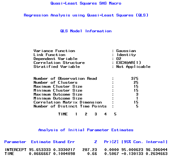
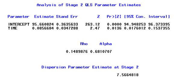
The first page describes the overall model information and initial parameter estimates using PROC GENMOD. Next SAS outputs are the stage 1 estimates with the corresponding 15 × 15 working correlation matrix and the 2 × 2 covariance matrix (time and intercept). For brevity, we show a part of the SAS output on the stage 2 estimates below:

For this particular data set, we assumed that the measurements were equally spaced in time, i.e. the difference between any consecutive time points is one. However, if the temporal gaps of consecutive measurements were not constant, the EXCHMarkov structure would be a more appropriate choice. The Markov structure would be selected by setting the option CORR=7 in %qlsmultcorr.

Note that in the output above, the maximum and minimum cluster sizes are both15, which indicate that all subjects had complete data. In addition, the maximum and minimum outcome sizes are both 3, which indicates that 3 methods of suctioning were available for each subject. In addition, there were5 distinct time points for the serial measurements that were measured on each of 25 subjects. Note also that the estimated values of ρ and of α were approximately 0.15 and 0.68, respectively. This suggests that the correlation within the serial measurements of each method over time was greater than the correlation between methods at each measurement occasion. The final (stage two) estimated regression coefficient for time was small, but did differ significantly from zero (p-value = 0.0136), which suggests that there was a small but statistically significant increase in suctioning values over time for these subjects.

Next, to demonstrate application of our software for unbalanced data, we randomly dropped 25 percent of the measurements from the oxygen data set. The smaller data set is named oxygen small. txt and is also available for download on the website https://dbe.med.upenn.edu/biostat-research/ladp#_Software.In the original data set, 25 of the subjects had 15 measurements that represented 5 measurements collected on each of 3 types of outcomes. In the smaller data set, 0 subjects have all 15measurements; 2 subjects have 14 measurements; 5 subjects have 13measurements; 3 subjects have 12 measurements; 8 subjects have 11measurements; 3 subjects have 10 measurements; 2 subjects have 9measurements; 1 subject has 8 measurements; and 1 subject has 7measurements. For this data set we specified an EXCH MARKOV structure.

The following codes can be used to analyze the unbalanced data which models O2 over TIME with the $\otimes$ Markov structure:

Data oxygen small;

infile"D,\oxygen small.txt" delimiter = "," ;

input ID TIME TYPE O2 FAMILY HIGH;

run;

Where we assume that the oxygen small data set is stored in D directory.

%qlsmultcorr (DATA=OXYGEN SMALL, Y=O2, X=TIME, TIME=TIME, ID=ID, OUTCOME=TYPE, LINK=1, CORR=7);

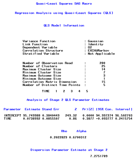
A part of the SAS output including the model information and the stage 2 estimates after executing the code above is below:

Results obtained for the EXCHMarkov structure are identical to those that we would have obtained for the EXCHAR1 structure. This follows from the fact that we assumed that the timings for the repeated measurements of each method were (1,2,3,4,5) for subjects with complete data and theAR1 and Markov structure are identical for these timings.(However, the results would not be the same for the AR1 and Marko structures if the planned timings for subjects with complete data differed from (1,2,3,4,5), e.g. if the planned timings for subjects with complete data were (1,2,4,10,20). Recall also that the correlation structure for subjects with missing observations is represented by a sub-matrix of the 15 × 15 correlation structure for subjects with complete data.

Note that in the output above, the number of observations read is now 280, which is approximately 75 percent of the previous sample size of 375. The maximum and minimum cluster sizes are now 14 and7, which indicates that no subjects had complete data. In addition, the maximum and minimum outcome sizes are now 3 and 1, which indicates that 3 methods of suctioning were available for some subjects, while some subjects had only one observed method of suctioning. In addition, there were 5 distinct time points for the serial measurements that were measured on each of 25 subjects. Therefore, no subject was totally dropped from the analysis.

Note also that the estimated values of ρ and of α were approximately 0.20 and 0.67, respectively. The estimated correlations were therefore similar for the balanced and unbalanced data sets. The final (stage two) estimated regression coefficient for time were also similar for the balanced and unbalanced data, but the regression coefficient for time did not differ significantly from zero for the smaller data set (p-value=0.3877) which may be due to the reduced power for the smaller data set.

It is also interesting to note that although no subject in the reduced data set had 15 measurements, the dimension of the correlation matrix was 15. This is because there were 3 distinct values (1,2,3) for the outcome variable and 5 distinct values(1,2,3,4,5) for the timings. The working correlation structure for each subject was a sub-matrix of this 15 × 15 working correlation structure.

Finally, we note that in Kim et al.,¹⁵ we allow for stratification on an additional variable that is nested within subjects by implementing different KP correlation structure for each stratum of the additional variable. For example, suppose the oxygen data contains patients who are treated with three methods of suctioning an endotracheal tube at several different intensive care units. In such case, it may be reasonable to use EXCH to describe the between-subject correlation within a total of m intensive care unit (ICU), and a common correlation AR1 for within-subject correlation over time. Thus, the correlation structure becomes as our reasonable working guess for the overall correlation structure stratified on each ICU. The following code implements the KP correlation structure stratified on the variable ICU:
% qlsmultcorr (DATA=OXYGEN, Y=O2, X=TIME, TIME=TIME, ID=ID, OUTCOME=TYPE, STRATUM=ICU, LINK=1, CORR=9);

Where ICU takes its value 1,2,…,m. For structure, %qlsmultcorr implements it with an option CORR=10, i.e.

% qlsmultcorr (DATA=OXYGEN, Y=O2, X=TIME, TIME=TIME, ID=ID, OUTCOME=TYPE, STRATUM=ICU, LINK=1, CORR=10)

%qlsmultcorr can fit a model to longitudinal data using the method of quasi-least squares for both single and (unbalanced) multiple outcomes described in Kim et al.¹⁵ %qlsmultcorr inapplicable for data that follow the normal, Bernoulli, or Poisson distribution with the AR1, Markov, equicorrelated, tri-diagonal, EXCH AR1, EXCH EXCH, EXCH Markov, EXCH Tri-diagonal, stratified EXCH AR1, and stratified EXCH EXCH structures. In particular, %qlsmultcorr can be applied for analysis of multi-outcome longitudinal data that are not balanced within clusters, due to the fact that some measurements are missing in a study that planned for an equal number of measurements to be collected on each of several outcomes on each subject.

This is an advantage over other existing software ¹⁵ in the presence of missing data, e.g. due to missing at least one of the outcome measurements at a particular visit within a subject"s longitudinal follow-up. In such a case, the %qlsmultcorr macro will model all the data, whereas other currently available software for QLS requires the deletion of all the outcome measurements for that corresponding visit in order to achieve balance prior to the analysis. The subsequent loss of information, due to the deletion of some data, may lead to inaccurate results in the analysis, and may also result in a loss of efficiency in testing the regression parameters.

%qlsmultcorr can also be used to analyze serial measurements that were collected on people within geographic regions (or clusters). However, we assume that the pair wise correlations within people in a region are equal at each measurement occasion; this assumption might be reasonable if we only know whether or not a subject resides within a particular region. For example, we might know the census tract in which each person resides. However, if we have more detailed information on the location of each person with each census tract, then the assumption of exchangeable correlations might be replaced with an assumed pattern of association that takes the distance between residences into account; such an extension is beyond the scope of this manuscript.

Further updates of %qlsmultcorr will be made to allow for implementation of other structures that are not currently available for GEE, including the KP structure based on the familial structure, KP structures which account for three or more sources of correlation, and structures that account for the geographic distance between people within a geographic region. It will also be of interest to develop and compare existing methods for selection of a working correlation structure and for assessment of goodness of fit of QLS (and GEE) models.

Authors declare that there is no conflict of interest

None.

1. Liang KY, Zeger SL. Longitudinal data analysis using generalized linear models. Biometrika. 1986;73(1):13–22.
2. Shults J, Morrow AL. Use of quasi–lease squares to adjust for two levels of correlation. Biometrics. 2002;58(3):521–530.
3. Galecki AT. General class of covariance structures for two or more repeated factors in longitudinal data analysis. Communications in Statistics. 1994;23(11):3105–3120.
4. Naik D, Rao S. Analysis of multivariate repeated measures data with a Kronecker product structured covariance matrix. Journal of Applied Statistics. 2001;28(1):91–105.
5. Roy A, Khattree R Testing the hypothesis of a Kroneckar product covariance matrix in multivariate repeated measures data. Statistics and Data Analysis. 2005;1:1–11.
6. Lu N, Zimmerman DL. The likelihood ratio test for a separable covariance matrix. Statistics and Probability Letters. 2005;73(4):449–457.
7. Roy A. A New classification rule for incomplete doubly multivariate data using mixed effects model with performance comparisons on the imputed data. Stat Med. 2006;25(10):1715–1728.
8. Roy A, Leiva R. Discrimination with jointly equicorrelated multi–level multivariate data. Advances in Data Analysis and Classification. 2007;1(3):175–199.
9. Chaganty NR. An alternative approach to the analysis of longitudinal data via generalized estimating equations. Journal of Statistical Planning and Inference. 1997;63(1):39–54.
10. Shults J, Chaganty NR. Analysis of serially correlated data using quasi-least squares. Biometrics. 1998;54:1622–1630.
11. Chaganty NR, Shults J. On eliminating the asymptotic bias in the quasi-least squares estimate of the correlation parameter. Journal of Statistical Planning and Inference. 1999;76(1–2):145–161.
12. Shults J, Morrow AL. Use of quasi–least squares to adjust for two levels of correlation. Biometrics. 2002;58(3):521–530.
13. Chaganty NR, Naik D. Analysis of multivariate longitudinal data using quasi–least squares. Journal of Statistical Planning and Inference. 2002;103(1–2):421–436.
14. Shults J, Whitt M, Kumanyika S. Analysis of data with multiple sources of correlation in the framework of generalized estimating equations. Stat Med. 2004;23(20):3209–3226.
15. Shults J, Ratcliffe S. Analysis of multi–level correlated data in the framework of generalized estimating equations via xtmultcorr procedures in Stata and qls Functions in Matlab. Statistics and Its Interface. 2009;2:187–196.
16. StataCorp. Stata Statistical Software: Release 13, College Station. Texas: Stata Corp LP; 2013.
17. MathWorks. MATLAB version7.10. Massachusetts: Natick; 2010.
18. Ratcliffe S, Shults J. GEEQBOX: A MATLAB toolbox for implementation of quasi–least squares and generalized estimating equations. Journal of Statistical Software. 2008;25(14):1–13.
19. Kim H, Shults J, Patterson S. Analysis of adverse events in drug safety: A multivariate approach using stratified quasi–least squares. USA: UPenn Biostatistics Working Papers: Working Paper; 2008.p. 29.
20. SAS Institute Inc. SAS/STAT Software, Version9.2. Cary. USA: North Carolina; 2003.
21. Weissfeld L, Kshirsagar A. A modified growth curve model and its application to clinical studies. Australian and New Zealand Journal of Statistics. 1992;34(2):161–168.
22. Kim H, Shults J. %QLS: A SAS macro for analysis of Correlated data using quasi–least squares. Journal of Statistical Software. 2010;35(2):1–22.
23. Davis CS. Statistical methods for the analysis of repeated measurements. Verlag: Springer; 2002.