Research Article Volume 13 Issue 1
An extended Suja distribution with statistical properties and applications
Rama Shanker,1 
shankerrama2009@gmail.com
Ronodeep Das,1 Kamlesh Kumar Shukla2
1 Department of Statistics, Assam University, Silchar, Assam, India
2 Department of Statistics, Jaypee Institute of Information Technology, Noida, India
Correspondence: Rama Shanker, Department of Statistics, Assam University, Silchar, India
Received: January 25, 2024 | Published: March 5, 2024
Citation: Shanker R, Das R, Shukla KK. An extended Suja distribution with statistical properties and applications. Biom Biostat Int J. 2024;13(1):16-21. DOI: 10.15406/bbij.2024.13.00409
Download PDF
Abstract
An extended Suja distribution, of which one parameter Suja distribution is a particular case, has been proposed. Important statistical properties of the proposed distribution based on moments, skewness, kurtosis, index of dispersion, hazard rate function, mean residual life function, stochastic ordering, mean deviations, Renyi entropy measures, and stress-strength reliability have been derived and studied. The method of moments and the method of maximum likelihood for estimating parameters have been discussed. A simulation study has been presented to know the performance of maximum likelihood estimates. Applications and goodness of fit of the proposed distribution with two real datasets have been presented.
Keywords: Suja distribution, statistical properties, parameters estimation, Goodness of fits
Introduction
The search for an appropriate statistical distribution for modeling of lifetime data is very challenging because the lifetime data are stochastic in nature. Statistical distributions are needed for modeling of lifetime data in engineering, medical science, demography, social sciences, physical sciences, finance, insurance, demography, social sciences, literature etc and during recent decades several researchers in statistics and mathematics tried to introduce lifetime distributions. In the exploration for a new lifetime distribution which can be useful to model lifetime data, Shanker1 proposed a one parameter distribution named Suja distribution defined by its probability density function (pdf) and cumulative distribution function (cdf)
(1.1)
(1.2)
Length- biased Suja distribution, power length-biased Suja distribution and weighted Suja distribution have been proposed and studied by Al-Omari and Alsmairan,2 Al-Omari et al.3 and Alsmairan et al.4 respectively. Todoka et al.5 have studied on the cdf of various modifications of Suja distributions and discussed their applications in the field of the analysis of computer- viruses’ propagation and debugging theory.
The main purpose of proposing an extended Suja distribution is to see the impact of additional parameter in the distribution over one parameter and other two-parameter distributions. Various descriptive measures, reliability properties and estimation parameters using both the method of moments and the method of maximum likelihood have been discussed. The applications and the goodness of fit of the distribution with two real lifetime datasets have been presented.
An extended Suja distribution
Taking the convex combination of exponential (θ) distribution and gamma (5,θ) distribution with mixing proportion
, the pdf of extended Suja distribution can be expressed as
(2.1)
We would call this a two-parameter Suja distribution (TPSD). The corresponding cdf and survival function of TPSD are thus obtained as
(2.2)
.
At α=1, TPSD reduces to Suja distribution. Also, for α=∞, TPSD reduces to exponential distribution. The pdf and the cdf of TPSD for varying values of parameters are shown in the Figures 1 & 2 respectively.
Measures based on moments
The rth moment about origin (raw moment)
of TPSD can be obtained as
Thus first four raw moments of TPSD can be expressed as
,
,
and
.
The central moments of TPSD are thus obtained as
The descriptive measures based on moments of TPSD such as coefficient of variation (C.V), coefficient of skewness
, coefficient of kurtosis
and index of dispersion
are obtained as
The behaviors of these descriptive measures are shown in the Figures 3-6 respectively.

Figure 3 Coefficient of variation of TPSD.

Figure 4 Coefficient of skewness of TPSD.

Figure 5 Coefficient of kurtosis of TPSD.

Figure 6 Index of dispersion of TPSD.
Reliability measures
The hazard rate function h(x) and the mean residual life function m(x) of a random variable X having pdf f(x) and cdf F(x) are defined as
and
.
Thus h(x) and m(x) of the TPSD are obtained as
and .
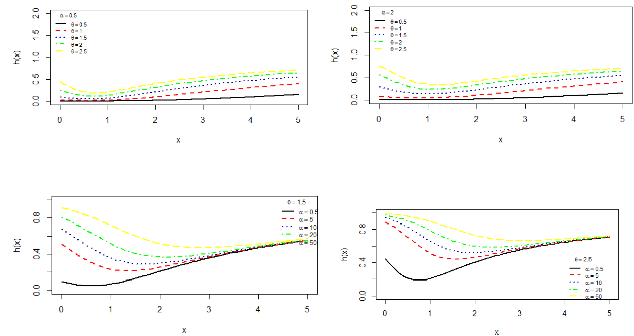
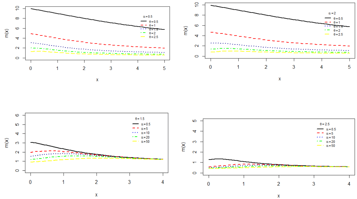
The h(x) and m(x) of TPSD are shown in Figures 7 & 8 respectively.

Figure 7 Hazard rate function of TPSD.

Figure 8 Mean residual life function of TPSD.
Mean deviations
The mean deviation about the mean and the mean deviation about the median are defined as
and
, respectively,
where
and
.
We have
Using above expressions and after little simplifications, the mean deviation about mean,
and the mean deviation about median,
of TPSD are obtained as
.
Order statistics
Let
denote the order statistics corresponding to random sample
. The pdf and the cdf of the kth order statistic, say
are given by
and
The pdf and the cdf of the kth order statistics of TPSD are thus obtained as
and
Stochastic orderings
Stochastic ordering of positive continuous random variables is an important tool for judging their comparative behavior. A random variable Y is said to be greater than a random variable X in the
- stochastic order
if
for all x
- hazard rate order
if
for all x
- mean residual life order
if
for all x
- Likelihood ratio order
if
decreases in x.
The well-known results due to Shaked and Shanthikumar6 for establishing stochastic ordering of distributions is
Using above results, we have shown in the following theorem that TPSD is ordered with respect to the strongest ‘likelihood ratio’ ordering.
Theorem: Let X∼ TPSD
and Y∼ TPSD
. If
, or
then
and hence
,
and
.
Proof: We have
Now
This gives
Thus, for
, or
,
. This means that
and hence
,
and
.
Renyi entropy measure
A measure of variation of uncertainty of a random variable X is known as Renyi entropy measure and given by Renyi.7 If X is a continuous random variable having pdf f(.), then Renyi entropy is defined as
,where
.
Thus, the Renyi entropy of TPSD can be obtained as
.
Stress-strength reliability
Let X and Y denote the strength and the stress of a component. The stress- strength reliability describes the life of a component whose random strength is subjected to a random stress. When
, the component fails instantly and the component will function satisfactorily till
. Therefore,
is the measure of component reliability and is known as stress-strength parameter. It has wide applications in engineering, biomedical science, social science etc.
Let X and Y are independent strength and stress random variables having TPSD with parameter
and
, respectively. Then, the stress-strength reliability R of TPSD can be obtained as
.
Estimation of parameters
Method of moments
Since TPSD has two parameters to be estimated, the first two moments about origin are required to estimate its parameters. We have
(Say)
Taking
, above equation becomes
(11.1.1)
Now, for real root of, the discriminant of the above equation should be greater than and equal to zero. That is
.
This means that the method of moments estimate is applicable if
, where
is the second moment about origin and
is the sample mean of the dataset. Now taking
in the expression for mean, we get the moment estimate
of
as
.
Using the moment estimate of
in
, we get the moment estimate
of α as
Thus the method of moment estimates
of parameters
of TPSD are given by
,
where
is the value of the quadratic equation in (11.1.1).
Method of maximum likelihood
Let
be a random sample of size n from TPSD (θ,α). Then the log- likelihood function of TPSD is given by
.
The maximum likelihood estimates
of parameters (θ,α) are the solution of the following log-likelihood equations
We have to use Fisher’s scoring method for solving these two log-likelihood equations because these two log-likelihood equations cannot be solved directly. We have
.
The following equations can be solved for MLEs
of (θ,α) of TPSD
where
and
are the initial values of θ and α, as given by the method of moments. These equations are solved iteratively till close estimates of parameters are obtained.
A simulation study
A simulation study has been carried out to check the performance of maximum likelihood estimates by taking sample sizes (n = 20,40,60,80) for values of
and
and 4. Acceptance and rejection method is used to generate random number for data simulation using R-software. The process was repeated 1,000 times for the calculation of Average Bias error (ABE) and MSE (Mean square error) of parameters θ and α are presented in Tables 1 &2 respectively. For the TPSD decreasing trend has been observed in ABE and MSE as the sample size increases and this shows that the performance of maximum likelihood estimators is quite good and consistent.
|
Sample
|
θ |
ABE(θ)
|
MSE (θ)
|
ABE (α)
|
MSE (α)
|
|
20
|
0.5
|
0.0323
|
0.02083
|
0.0645
|
0.7180
|
|
1.0
|
0.0073
|
0.0010
|
0.1145
|
0.2621
|
|
1.5
|
-0.0177
|
0.0063
|
0.0645
|
0.0831
|
|
2.0
|
-0.0427
|
0.0365
|
0.0144
|
0.0041
|
|
40
|
0.5
|
0.0168
|
0.0113
|
-0.0074
|
0.1210
|
|
1.0
|
0.0043
|
0.0007
|
0.0175
|
0.0122
|
|
1.5
|
-0.0081
|
0.0026
|
-0.0074
|
0.0022
|
|
2.0
|
-0.0206
|
0.0170
|
-0.0324
|
0.0422
|
|
60
|
0.5
|
0.0098
|
0.0058
|
-0.0011
|
0.0982
|
|
1.0
|
0.0015
|
0.0001
|
0.0143
|
0.0154
|
|
1.5
|
-0.0067
|
0.0027
|
-0.0011
|
0.0008
|
|
2.0
|
-0.0151
|
0.0136
|
-0.0178
|
0.0191
|
|
80
|
0.5
|
0.0057
|
0.0026
|
0.0292
|
0.2932
|
|
1.0
|
-0.0004
|
0.0001
|
0.0417
|
0.1397
|
|
1.5
|
-0.0067
|
0.0035
|
0.0292
|
0.0686
|
|
2.0
|
-0.0129
|
0.01342
|
0.0167
|
0.0225
|
Table 1 ABE and MSE of parameters at fixed value α=0.5
|
Sample
|
θ |
ABE (θ)
|
MSE (θ)
|
ABE (α)
|
MSE (α)
|
|
20
|
0.5
|
0.0156
|
0.0048
|
0.0387
|
0.5365
|
|
1.0
|
-0.0093
|
0.0017
|
0.0887
|
0.1576
|
|
1.5
|
-0.0343
|
0.0236
|
0.0387
|
0.0300
|
|
2.0
|
-0.0593
|
0.0704
|
-0.0112
|
0.0025
|
|
40
|
0.5
|
0.0168
|
0.0113
|
-0.0074
|
0.1210
|
|
1.0
|
0.0043
|
0.0007
|
0.01750
|
0.0122
|
|
1.5
|
-0.0081
|
0.0026
|
-0.0074
|
0.0022
|
|
2.0
|
-0.0206
|
0.0170
|
-0.0324
|
0.0422
|
|
60
|
0.5
|
0.0100
|
0.0060
|
-0.0064
|
0.0745
|
|
1.0
|
0.0016
|
0.0001
|
0.0102
|
0.0063
|
|
1.5
|
-0.0066
|
0.0026
|
-0.0064
|
0.0024
|
|
2.0
|
-0.0149
|
0.0134
|
-0.0230
|
0.0319
|
|
80
|
0.5
|
0.0057
|
0.0026
|
0.0306
|
0.3063
|
|
1.0
|
-0.0004
|
0.0017
|
0.0431
|
0.1488
|
|
1.5
|
-0.0068
|
0.0036
|
0.0306
|
0.0750
|
|
2.0
|
-0.0129
|
0.0134
|
0.0181
|
0.0262
|
Table 2 ABE and MSE of parameters at fixed value of α=4
Applications
The goodness of fit of TPSD along with its comparison with one parameter Suja distribution and two-parameter lifetime distributions including quasi Lindley distribution (QLD) of Shanker and Mishra,8 a two-parameter Lindley distribution (TPLD-I b) of Shanker and Mishra,9 a two-parameter Lindley distribution (TPLD-II) of Shanker et al.10 for two real lifetime datasets relating to failure times have been discussed. The applications of the TPSD can also be extended to model the survival times of patients suffering from serious disease in medical sciences. The pdf and the cdf of these distributions are presented in the following Table 3.
|
Distributions
|
pdf
|
Cdf
|
|
TPLD-I
|
|
|
|
TPLD-II
|
|
|
|
QLD
|
|
|
Table 3 pdf and the cdf of two-parameter distributions
The two datasets considered for testing the goodness of fit of TPSD over other one parameter and two-parameter lifetime distributions are as follows:
Dataset 1: The positively skewed data relating to the accelerated life testing of item (
) with changes in stress from 100 to 150 at time
, available in Murthy et al (2004).
0.032, 0.035, 0.104, 0.169, 0.196, 0.260, 0.326, 0.445, 0.449, 0.496, 0.543, 0.544, 0.577, 0.648, 0.666, 0.742, 0.757, 0.808, 0.857, 0.858, 0.882, 1.005, 1.025, 1.472, 1.916, 2.313, 2.457, 2.530, 2.543, 2.617, 2.835, 2.940, 3.002, 3.158, 3.430, 3.459, 3.502, 3.691, 3.861, 3.952, 4.396, 4.744, 5.346, 5.479, 5.716, 5.825, 5.847, 6.084, 6.127, 7.241, 7.560, 8.901, 9.000, 10.482, 11.133.
Dataset 2: The positively skewed failure time data (
), available in Murthy et al (2004).
0.13, 0.62, 0.75, 0.87, 1.56, 2.28, 3.15, 3.25, 3.55, 4.49, 4.50, 4.61, 4.79, 7.17, 7.31, 7.43, 7.84, 8.49, 8.94, 9.40, 9.61, 9.84, 10.58, 11.18, 11.84, 13.28, 14.47, 14.79, 15.54, 16.90, 17.25, 17.37, 18.69, 18.78, 19.88, 20.06, 20.10, 20.95, 21.72, 23.87.
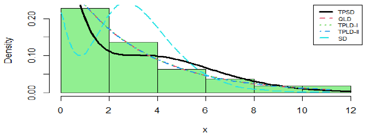
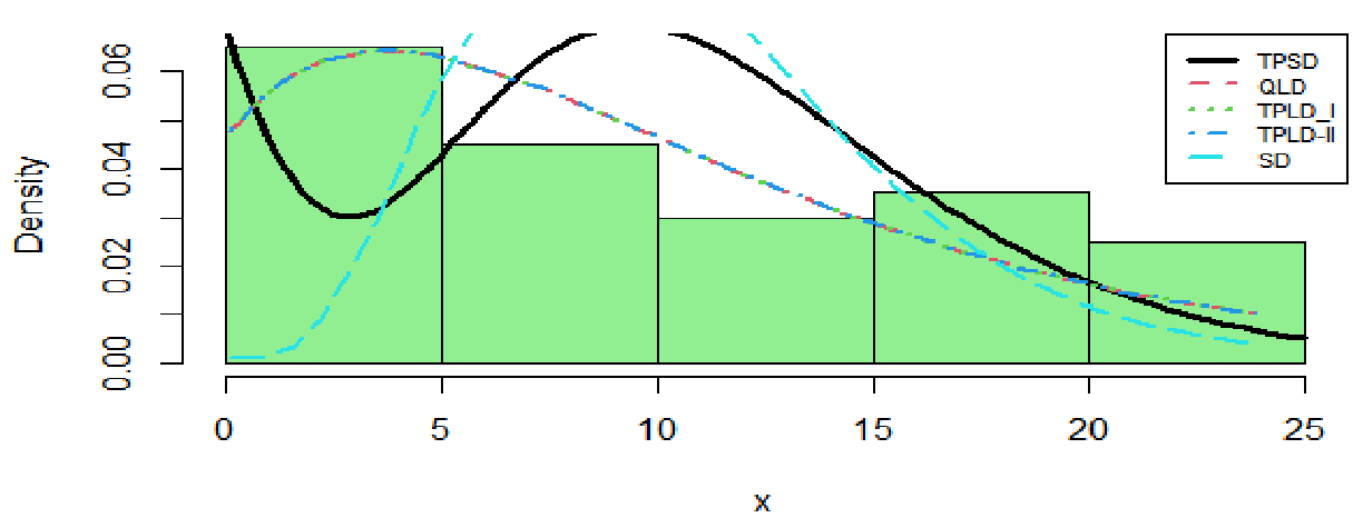
The corresponding maximum likelihood estimates of parameters along with -2logL, AIC, kolmogorov-Smirnov (K-S) and p-values of the considered datasets for the given distributions are presented in Table 4 & 5, respectively. The fitted plots of the distributions for the considered two datasets have been shown in Figures 9 & 10 respectively. The goodness of fit in Tables 4 & 5 and the fitted plots in Figures 9 & 10 shows that TPSD gives much closer fit for the considered datasets in Table 4 while in Table 5 TPLD-1 gives better fit over other distributions. Therefore, it can be concluded that TPSD and TPLD-1 can be considered the best distributions for lifetime data.
|
Distributions
|
ML estimates
|
-2logL |
AIC
|
K-S
|
p-value
|
|
|
θ
|
α
|
|
|
|
|
|
TPSD
|
0.9563
|
32.1684
|
226.65
|
230.65
|
0.086
|
0.774
|
|
QLD
|
0.3848
|
5.19455
|
231.44
|
235.44
|
0.135
|
0.244
|
|
TPLD-I
|
0.3907
|
11.6595
|
231.45
|
235.45
|
0.136
|
0.235
|
|
TPLD-II
|
0.383
|
0.07082
|
231.44
|
235.44
|
0.134
|
0.246
|
|
SD
|
1.4504
|
……..
|
265.86
|
267.86
|
0.282
|
0.0002
|
Table 4 ML estimates of the parameters of distributions and values of
for data set 1.
|
Distributions
|
ML estimates
|
-2logL
|
AIC
|
K-S
|
p-value
|
|
|
θ
|
α
|
|
|
|
|
|
TPSD
|
0.4175
|
158.423
|
262.10
|
266.10
|
0.136
|
0.406
|
|
QLD
|
0.16453
|
0.3914
|
263.24
|
267.24
|
0.107
|
0.708
|
|
TPLD-I
|
0.16456
|
2.3745
|
263.25
|
263.25
|
0.106
|
0.711
|
|
TPLD-II
|
0.16453
|
0.42038
|
263.24
|
267.24
|
0.107
|
0.709
|
|
SD
|
0.4778
|
……..
|
301.17
|
303.17
|
0.24
|
0.015
|
Table 5 ML estimates of the parameters of distributions values of
for data

Figure 9 Fitted plots of distributions for data set1.

Figure 10 Fitted plots of distributions for datasets 2.
Conclusion
In this paper, a two-parameter Suja distribution has been proposed by introducing an additional parameter in one parameter Suja distribution to see its effect regarding goodness of fit over Suja distribution and other two-parameter lifetime distributions. Its various descriptive measures based on moments and reliability properties have been discussed. The estimation of parameters using method of moments and maximum likelihood method has been discussed. A simulation study has been presented to know the performance of maximum likelihood estimates. The goodness of fit of the proposed distribution has been presented with two real lifetime datasets.
Acknowledgments
Authors are grateful to the editor in chief and the anonymous reviewer for some minor comments which improved both the quality and the presentation.
Conflicts of interest
Funding
References
- Shanker R. Suja distribution and its application. International Journal of Probability and Statistics. 2017;6(2):11–19.
- Al-Omari AI, Alsmairam I.K. Length-biased Suja distribution and Its application, Journal of Applied Probability and Statistics. 2019;14(3):95–116.
- Al-Omari AI, Alhyasat IK, Abu B.M.A. Power length-biased Suja distribution –properties and application. Electronic Journal of Applied Statistical Analysisl. 2019;12(2):429–452.
- Alsmairan IK, Al-Omari AI. Weighted Suja distribution with application to ball bearings data, Life Cycle Reliability and Safety Engineering. 2020;9:195–211.
- Todorka T, Anton I, Asen R, et al. Comments on some modification of Suja Cumulative Functions with applications to the theory of computer viruses propagation. International Journal of Differential Equations and Applications. 2020;19(1):83–95.
- Shaked M, Shanthikumar JG. Stochastic orders and their applications. Academic Press; New York. 1994.
- Renyi A. On measures of entropy and information. Berkeley Symp on Math Statist Prob. 1961;1:547–561.
- Shanker R, Mishra A. A quasi Lindley distribution. African Journal of Mathematics and Computer Science Research. (2013 a);6(4):64– 71.
- Shanker R, Mishra A. A two-parameter Lindley distribution. Statistics in Transition New Series. 2013(b);14(1):45–56.
- Shanker R, Sharma S, Shanker R. A two -parameter Lindley distribution for modeling waiting and survival times data. Applied Mathematics. 2013;4(2):363–368.
- Murthy DNP, Xie M, Jiang R. Weibull Models. John Wiley& sons Inc; Hoboken. 2004.
- Bonferroni CE. Elementi di Statistca generale. Seeber; Firenze. 1930.

©2024 Shanker, et al. This is an open access article distributed under the terms of the,
which
permits unrestricted use, distribution, and build upon your work non-commercially.


