In this paper, a new one parameter life lime distribution has been proposed and named Pranav distribution. Its statistical and mathematical properties have been derived and its stochastic ordering, mean deviations, Bonferroni and Lorenz curves, order statistics, Renyi entropy measure and stress–strength reliability have been discussed. A Simulation study of proposed distribution has also been discussed. For estimating its parameter method of moments and method of maximum likelihood estimation have been discussed. Goodness of fit of proposed distribution has been presented and compared with other lifetime distributions of one parameter.

Keywords: estimation of parameters, mean deviation, moments, order statistics, reliability measures, renyi entropy measure, stochastic ordering, stress–strength reliability

Many researchers have been proposed many distributions of one parameter as well as two parameters for modeling life time data. Some of them are giving good results for different data sets from biological and engineering which are considered as life time distribution. But some of them are not giving good results for all the data sets from biological and engineering such as Lindley distribution proposed by Lindley¹ Akash and Shanker distributions proposed by Shanker^2,3 and Ishita distribution proposed by Shanker.⁴ These distributions are giving good fit over exponential distribution whereas Akash distribution proposed by Shanker² has been applied on biological data and mentioned the superiority over Lindley distribution and Exponential distribution.

The detailed study about its mathematical properties, estimation of parameter and application has been shown in their paper. Sujatha distribution proposed by Shanker⁵ has also been applied on real life time data from biological and engineering. Its mathematical and statistical properties has also been discussed in that paper and showed on some selected data set, better than Lindley and Exponential distribution.

Ghitany⁶ reported in their paper that Lindley distribution is superior to exponential distribution with reference to data related the waiting time before service of the bank customers. In this regard, author interest was to propose new life time distribution which may give good fit in compare to other life time distribution. That is main motivation to propose a new life distribution and applied on biological data.

Therefore, searching a new life time distribution which may be better than Lindley, Exponential, Ishita, Shanker, Sujatha and Akash distribution. It is describe as below:

One parameter life time distribution having parameters $\theta$is defined by its pdf

$f\left(x;\theta \right)=\frac{{\theta }^4}{{\theta }^4+6}\left(\theta +x^3\right)e^{-\theta x};x>0,\theta >0$(1.1)

The pdf (1.1) would call ‘Pranav distribution’ which is a mixture of two–distributions , exponential distribution having scale parameter $\theta$ and gamma distribution having shape parameter 4 and scale parameter,  and their mixing proportions of $\theta$ $\frac{{\theta }^4}{\left({\theta }^4+6\right)}$and $\frac{6}{\left({\theta }^4+6\right)}$respectively.

$$f_2\left(x;\theta \right)=p{g}_1\left(x;\theta \right)+(1-p)g_2\left(x;\theta ,4\right)$$

Where $p=\frac{{\theta }^4}{\left({\theta }^4+6\right)},g_1\left(x\right)=\theta e^{-\theta x}$and $g_2\left(x\right)=\frac{{\theta }^4{x}^3{e}^{-\theta x}}{6}$

The corresponding cumulative distribution function (cdf) of (1.1) is given by

$F\left(x;\theta \right)=1-\left[1+\frac{\theta x\left({\theta }^2{x}^2+3\theta x+6\right)}{{\theta }^4+6}\right]e^{-\theta x};x>0,\theta >0$(1.2)

In this study, new one parameter life time distribution has been proposed and named Pranav distribution. Moment and its related measures have been discussed. Its hazard rate function, mean residual life function, stochastic ordering, mean deviations, Bonferroni and Lorenz curves, order statistics, Renyi entropy measure and stress–strength reliability have been discussed. A simulation study of proposed distribution has also been discussed. Both the method of moments and the method of maximum likelihood estimation have been discussed for estimating the parameter of Pranav distribution. The goodness of fit of the Pranav distribution has been presented and the fit has also been compared with other lifetime distributions of one parameter.

Graphs of the pdf and the cdf of Pranav distribution for varying values of parameter are presented in Figure 1 & 2.

Figure 1 Pdf plots of Pranav distribution of varying values of parameter θ.

Figure 2 Cdf plots of Pranav distribution of varying values of parameter θ.

The $r$^th moment about origin of Pranav distribution can be obtained as

${\mu }_r{}^{\prime }=\frac{r!\left[{\theta }^4+\left(r+1\right)\left(r+2\right)\right]\left(r+3\right)}{{\theta }^r\left({\theta }^4+6\right)};r=1,2,3,\mathrm{...}$ (2.1)

Thus the first four moments about origin of Pranav distribution are given by

${\mu }_1{}^{\prime }=\frac{{\theta }^4+24}{\theta \left({\theta }^4+6\right)}$, ${\mu }_2{}^{\prime }=\frac{2({\theta }^4+60)}{{\theta }^2\left({\theta }^4+6\right)}$,

${\mu }_3{}^{\prime }=\frac{6({\theta }^4+120)}{{\theta }^3\left({\theta }^4+6\right)}$,${\mu }_4{}^{\prime }=\frac{24({\theta }^4+210)}{{\theta }^4\left({\theta }^4+6\right)}$

Using above raw moments about origin, central moments of Pranav distribution are thus derived as

$${\mu }_2=\frac{({\theta }^8+84{\theta }^4+144)}{{\theta }^2{\left({\theta }^4+6\right)}^2}$$

$${\mu }_3=\frac{2({\theta }^{12}+198{\theta }^8+324{\theta }^4+864)}{{\theta }^3{\left({\theta }^4+6\right)}^3}$$

$${\mu }_4=\frac{9({\theta }^{16}+312{\theta }^{12}+2304{\theta }^8+10368{\theta }^4+10368)}{{\theta }^4{\left({\theta }^4+6\right)}^4}$$

The coefficient of variation $\left(C.V\right)$, coefficient of skewness $\left(\sqrt{{\beta }_1}\right)$, coefficient of kurtosis $\left({\beta }_2\right)$ and index of dispersion $\left(\gamma \right)$ of Pranav distribution are obtained as

$$C.V=\frac{\sigma }{{\mu }_1{}^{\prime }}=\frac{\sqrt{({\theta }^8+84{\theta }^4+144)}}{\left({\theta }^4+24\right)}$$

$$\sqrt{{\beta }_1}=\frac{{\mu }_3}{{\mu }_2{}^{3/2}}=\frac{2({\theta }^{12}+198{\theta }^8+324{\theta }^4+864)}{{\left({\theta }^8+84{\theta }^4+144\right)}^{3/2}}$$

$${\beta }_2=\frac{{\mu }_4}{{\mu }_2{}^2}=\frac{9({\theta }^{16}+312{\theta }^{12}+2304{\theta }^8+10368{\theta }^4+10368)}{{\left({\theta }^8+84{\theta }^4+144\right)}^2}$$

$$\gamma =\frac{{\sigma }^2}{{\mu }_1{}^{\prime }}=\frac{({\theta }^8+84{\theta }^4+144)}{\theta ({\theta }^4+6)({\theta }^4+24)}$$

To study the nature of C.V, $\sqrt{{\beta }_1}$, ${\beta }_2$, and of Pranav distribution, graphs of C.V, $\sqrt{{\beta }_1}$, ${\beta }_2$, and $\gamma$ of Pranav distribution have been drawn for varying values of the parameters and presented in Figure 3.

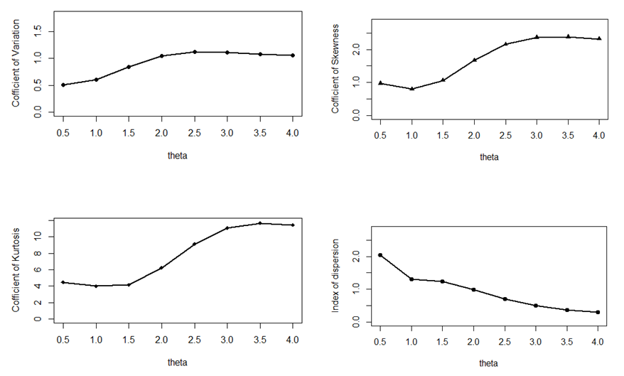
Figure 3 CV, $\sqrt{{\beta }_1}$, ${\beta }_2$and $\gamma$ of Pranav distribution.

Let X be a continuous random variable with pdf $f\left(x\right)$ and cdf $F\left(x\right)$. The hazard rate function (also known as the failure rate function) and the mean residual life function of are respectively defined as

$h\left(x\right)=\frac{f\left(x\right)}{1-F\left(x\right)}$ (3.1)

$m\left(x\right)=E\left[X-x|X>x\right]=\frac{1}{1-F\left(x\right)}{\displaystyle {\int }_x^{\infty }\left[1-F\left(t\right)\right]}dt$ (3.2)

The corresponding hazard rate function, $h\left(x\right)$ and the mean residual life function, $m\left(x\right)$ of Pranav distribution (1.1) are obtained as

$h\left(x\right)=\frac{{\theta }^4\left(\theta +x^3\right)}{\left({\theta }^3{x}^3+3{\theta }^2{x}^2+6\theta x+{\theta }^4+6\right)}$ (3.3)

and $m\left(x\right)=\frac{1}{\left({\theta }^3{x}^3+3{\theta }^2{x}^2+6\theta x+{\theta }^4+6\right)}{\displaystyle \underset{x}{\overset{\infty }{\int }}\left({\theta }^3{t}^3+3{\theta }^2{t}^2+6\theta t+{\theta }^4+6\right)e^{-\theta t}dt}$

$=\frac{\left({\theta }^3{x}^3+6{\theta }^2{x}^2+18\theta x+{\theta }^4+24\right)}{\theta \left({\theta }^3{x}^3+3{\theta }^2{x}^2+6\theta x+{\theta }^4+6\right)}$(3.4)

 It can be easily verified that $h\left(0\right)=\frac{{\theta }^5}{{\theta }^4+6}=f\left(0\right)$ and $m\left(0\right)=\frac{{\theta }^4+24}{\theta \left({\theta }^4+6\right)}={\mu }_1{}^{\prime }$.

The graph of $h\left(x\right)$ and $m\left(x\right)$ of Pranav distribution for varying values of parameter is shown in Figure 4&5 respectively.

Figure 4 h(x) of Pranav distribution for varying value of parameter θ.

Figure 5 m(x) of Pranav distribution for varying values of parameter θ.

Stochastic ordering of positive continuous random variables is crucial method for evaluating their comparative behavior. A random variable X is said to be smaller than a random variable Y in the

stochastic order $\left(X{\le }_{st}Y\right)$ if $F_X\left(x\right)\ge F_Y\left(x\right)$ for all $x$

hazard rate order $\left(X{\le }_{hr}Y\right)$ if $h_X\left(x\right)\ge h_Y\left(x\right)$ for all x

mean residual life order $\left(X{\le }_{mrl}Y\right)$ if $m_X\left(x\right)\le m_Y\left(x\right)$for all x

likelihood ratio order $\left(X{\le }_{lr}Y\right)$if $\frac{f_X\left(x\right)}{f_Y\left(x\right)}$decreases in x.

The following results due to Shaked⁷ are well known for establishing stochastic ordering of distributions

$$X{\le }_{lr}Y\Rightarrow X{\le }_{hr}Y\Rightarrow X{\le }_{mrl}Y$$

$$\underset{X{\le }_{st}Y}{\Downarrow }$$

The Pranav distribution is ordered with respect to the strongest ‘likelihood ratio ordering’ as established in the following theorem:

Theorem: Let X and Y follows Pranav distribution with parameters $\left({\theta }_1\right)$ and $\left({\theta }_2\right)$ respectively. If ${\theta }_1\ge {\theta }_2$then $X{\le }_{lr}Y$ and hence $X{\le }_{hr}Y$, $X{\le }_{mrl}Y$ and $X{\le }_{st}Y$.

Proof: We have

$\frac{f_X\left(x;{\theta }_1\right)}{f_Y\left(x;{\theta }_2\right)}=\frac{{\theta }_1{}^4\left({\theta }_2{}^4+6\right)}{{\theta }_2{}^4\left({\theta }_1{}^4+6\right)}{e}^{-\left({\theta }_1-{\theta }_2\right)x}$$;x>0$

Now

$$\ln \frac{f_X\left(x;{\theta }_1\right)}{f_Y\left(x;{\theta }_2\right)}=\ln \left[\frac{{\theta }_1{}^4\left({\theta }_2{}^4+6\right)}{{\theta }_2{}^4\left({\theta }_1{}^4+6\right)}\right]-\left({\theta }_1-{\theta }_2\right)x$$

This gives $$\frac{d}{dx}\ln \frac{f_X\left(x;{\theta }_1\right)}{f_Y\left(x;{\theta }_2\right)}=-\left({\theta }_1-{\theta }_2\right)$$

 Thus if ${\theta }_1>{\theta }_2$or ${\theta }_1={\theta }_2$, $\frac{d}{dx}\ln \frac{f_X\left(x;{\theta }_1\right)}{f_Y\left(x;{\theta }_2\right)}<0$. This means that $X{\le }_{lr}Y$ and hence $X{\le }_{hr}Y$, $X{\le }_{mrl}Y$ and $X{\le }_{st}Y$.

The mean deviation about the mean and median are defined by

${\delta }_1\left(X\right)={\displaystyle \underset{0}{\overset{\infty }{\int }}\left|x-\mu \right|}f\left(x\right)dx$ and ${\delta }_2\left(X\right)={\displaystyle \underset{0}{\overset{\infty }{\int }}\left|x-M\right|}f\left(x\right)dx$, respectively, where $\mu =E\left(X\right)$and $M=\text{Median }\left(X\right)$. The measures ${\delta }_1\left(X\right)$and ${\delta }_2\left(X\right)$can be calculated using the following simplified relationships

$${\delta }_1\left(X\right)={\displaystyle \underset{0}{\overset{\mu }{\int }}\left(\mu -x\right)}f\left(x\right)dx+{\displaystyle \underset{\mu }{\overset{\infty }{\int }}\left(x-\mu \right)}f\left(x\right)dx$$

$$=\mu F\left(\mu \right)-{\displaystyle \underset{0}{\overset{\mu }{\int }}xf\left(x\right)dx}-\mu \left[1-F\left(\mu \right)\right]+{\displaystyle \underset{\mu }{\overset{\infty }{\int }}x}f\left(x\right)dx$$

$$=2\mu F\left(\mu \right)-2\mu +2{\displaystyle \underset{\mu }{\overset{\infty }{\int }}x}f\left(x\right)dx$$

$=2\mu F\left(\mu \right)-2{\displaystyle \underset{0}{\overset{\mu }{\int }}x}f\left(x\right)dx$(5.1)

and

$${\delta }_2\left(X\right)={\displaystyle \underset{0}{\overset{M}{\int }}\left(M-x\right)}f\left(x\right)dx+{\displaystyle \underset{M}{\overset{\infty }{\int }}\left(x-M\right)}f\left(x\right)dx$$

$=MF\left(M\right)-{\displaystyle \underset{0}{\overset{M}{\int }}xf\left(x\right)dx}-M\left[1-F\left(M\right)\right]+{\displaystyle \underset{M}{\overset{\infty }{\int }}x}f\left(x\right)dx$

$$=-\mu +2{\displaystyle \underset{M}{\overset{\infty }{\int }}x}f\left(x\right)dx$$

$=\mu -2{\displaystyle \underset{0}{\overset{M}{\int }}x}f\left(x\right)dx$(5.2)

Using pdf (1.1) and the mean of Pranav distribution, it can be written as:

${\displaystyle \underset{0}{\overset{\mu }{\int }}x}f\left(x;\theta \right)dx=\mu -\frac{\left\{{\theta }^5\mu +\left({\mu }^4+1\right){\theta }^4+4{\theta }^3{\mu }^3+12{\theta }^2{\mu }^2+24\theta \mu +24\right\}{e}^{-\theta \mu }}{\theta \left({\theta }^4+6\right)}$(5.3)

${\displaystyle \underset{0}{\overset{M}{\int }}x}f\left(x;\theta \right)dx=\mu -\frac{\left\{{\theta }^{5}M+\left(M^4+1\right){\theta }^4+4{\theta }^3{M}^3+12{\theta }^2{M}^2+24\theta M+24\right\}{e}^{-\theta M}}{\theta \left({\theta }^4+6\right)}$(5.4)

Using equations (5.1), (5.2), (5.3), and (5.4), the mean deviation about mean, ${\delta }_1\left(X\right)$and the mean deviation about median, ${\delta }_2\left(X\right)$of Pranav distribution are calculated as

${\delta }_1\left(X\right)=\frac{2\left\{{\theta }^4+{\theta }^3{\mu }^3+6{\theta }^2{\mu }^2+18\theta \mu +24\right\}{e}^{-\theta \mu }}{\theta \left({\theta }^4+6\right)}$(5.5)

${\delta }_2\left(X\right)=\frac{2\left\{{\theta }^{5}M+\left(M^4+1\right){\theta }^4+4{\theta }^3{M}^3+12{\theta }^2{M}^2+24\theta M+24\right\}{e}^{-\theta M}}{\theta \left({\theta }^4+6\right)}-\mu$(5.6)

The Bonferroni and Lorenz curves Bonferroni⁸ and Gini indices have important used in economics to study income and poverty of any state. It’s relevance also in other fields like reliability, demography, insurance and medicine. The Bonferroni and Lorenz curves are obtained as

$B\left(p\right)=\frac{1}{p\mu }{\displaystyle \underset{0}{\overset{q}{\int }}xf\left(x\right)}dx=\frac{1}{p\mu }\left[{\displaystyle \underset{0}{\overset{\infty }{\int }}xf\left(x\right)dx-}{\displaystyle \underset{q}{\overset{\infty }{\int }}xf\left(x\right)}dx\right]=\frac{1}{p\mu }\left[\mu -{\displaystyle \underset{q}{\overset{\infty }{\int }}xf\left(x\right)}dx\right]$ (6.1)

and $L\left(p\right)=\frac{1}{\mu }{\displaystyle \underset{0}{\overset{q}{\int }}xf\left(x\right)}dx=\frac{1}{\mu }\left[{\displaystyle \underset{0}{\overset{\infty }{\int }}xf\left(x\right)dx-}{\displaystyle \underset{q}{\overset{\infty }{\int }}xf\left(x\right)}dx\right]=\frac{1}{\mu }\left[\mu -{\displaystyle \underset{q}{\overset{\infty }{\int }}xf\left(x\right)}dx\right]$(6.2)

 respectively or equivalently.

$B\left(p\right)=\frac{1}{p\mu }{\displaystyle \underset{0}{\overset{p}{\int }}{F}^{-1}\left(x\right)}dx$(6.3) and $L\left(p\right)=\frac{1}{\mu }{\displaystyle \underset{0}{\overset{p}{\int }}{F}^{-1}\left(x\right)}dx$(6.4) respectively, where $\mu =E\left(X\right)$and $q=F^{-1}\left(p\right)$.

 The Bonferroni and Gini indices are thus defined as

$B=1-{\displaystyle \underset{0}{\overset{1}{\int }}B\left(p\right)}dp$(6.5) and $G=1-2{\displaystyle \underset{0}{\overset{1}{\int }}L\left(p\right)}dp$(6.6) respectively.

 Using pdf of Pranav distribution (1.1), it can be written

${\displaystyle \underset{q}{\overset{\infty }{\int }}xf\left(x;\theta \right)}dx=\frac{\left\{{\theta }^{5}q+{\theta }^4(q^4+1)+4{\theta }^3{q}^3+12{\theta }^2{q}^2+24\theta q+24\right\}{e}^{-\theta \mu }}{\theta \left({\theta }^4+6\right)}$ (6.7)

Now using equation (6.7) in (6.1) and (6.2),

$B\left(p\right)=\frac{1}{p}\left[1-\frac{\left\{{\theta }^{5}q+{\theta }^4(q^4+1)+4{\theta }^3{q}^3+12{\theta }^2{q}^2+24\theta q+24\right\}{e}^{-\theta \mu }}{\left({\theta }^4+6\right)}\right]$(6.8)

and $L\left(p\right)=1-\frac{\left\{{\theta }^{5}q+{\theta }^4(q^4+1)+4{\theta }^3{q}^3+12{\theta }^2{q}^2+24\theta q+24\right\}{e}^{-\theta \mu }}{\left({\theta }^4+6\right)}$(6.9)

 Now using equations (6.8) and (6.9) in (6.5) and (6.6), the Bonferroni and Gini indices of Pranav distribution are thus obtained as

$B=1-\frac{\left\{{\theta }^{5}q+{\theta }^4(q^4+1)+4{\theta }^3{q}^3+12{\theta }^2{q}^2+24\theta q+24\right\}{e}^{-\theta \mu }}{\left({\theta }^4+6\right)}$(6.10)

$G=\frac{2\left\{{\theta }^{5}q+{\theta }^4(q^4+1)+4{\theta }^3{q}^3+12{\theta }^2{q}^2+24\theta q+24\right\}{e}^{-\theta \mu }}{\left({\theta }^4+6\right)}-1$(6.11)

Order statistics

Let $X_1,X_2,\mathrm{...},X_n$be a random sample of size $n$from Pranav distribution (1.1). Let $X_{\left(1\right)}<X_{\left(2\right)}<\mathrm{...}<X_{\left(n\right)}$ denote the corresponding order statistics. The pdf and the cdf of the Kth order statistic, say $Y=X_{\left(k\right)}$are given by

$$f_Y\left(y\right)=\frac{n!}{\left(k-1\right)!\left(n-k\right)!}{F}^{k-1}\left(y\right){\left\{1-F\left(y\right)\right\}}^{n-k}f\left(y\right)$$

$$=\frac{n!}{\left(k-1\right)!\left(n-k\right)!}{\displaystyle \sum _{l=0}^{n-k}\left(\begin{array}{c}n-k\\ l\end{array}\right)}{\left(-1\right)}^l{F}^{k+l-1}\left(y\right)f\left(y\right)$$

 and

$$F_Y\left(y\right)={\displaystyle \sum _{j=k}^n\left(\begin{array}{c}n\\ j\end{array}\right)}{F}^j\left(y\right){\left\{1-F\left(y\right)\right\}}^{n-j}$$

$$={\displaystyle \sum _{j=k}^n{\displaystyle \sum _{l=0}^{n-j}\left(\begin{array}{c}n\\ j\end{array}\right)}\left(\begin{array}{c}n-j\\ l\end{array}\right)}{\left(-1\right)}^l{F}^{j+l}\left(y\right)$$

 respectively, for $k=1,2,3,\mathrm{...},n$.

 Thus, the pdf and the cdf of Kth order statistic of Pranav distribution (1.1) are obtained as

$$\begin{array}{l}{f}_Y\left(y\right)=\frac{n!{\theta }^4\left(\theta +x^3\right)e^{-\theta x}}{\left({\theta }^4+6\right)\left(k-1\right)!\left(n-k\right)!}{\displaystyle \sum _{l=0}^{n-k}\left(\begin{array}{c}n-k\\ l\end{array}\right)}{\left(-1\right)}^l\\ \times {\left[1-\frac{\left\{\theta x\left({\theta }^2{x}^2+3\theta x+6\right)+\left({\theta }^4+6\right)\right\}{e}^{-\theta x}}{({\theta }^4+6)}\right]}^{k+l-1}\end{array}$$

and

$$F_Y\left(y\right)={\displaystyle \sum _{j=k}^n{\displaystyle \sum _{l=0}^{n-j}\left(\begin{array}{c}n\\ j\end{array}\right)}\left(\begin{array}{c}n-j\\ l\end{array}\right)}{\left(-1\right)}^l{\left[1-\frac{\left\{\theta x\left({\theta }^2{x}^2+3\theta x+6\right)+\left({\theta }^4+6\right)\right\}{e}^{-\theta x}}{({\theta }^4+6)}\right]}^{j+l}$$

Renyi entropy measure

A popular entropy measure is given by Renyi entropy.⁹ If is a continuous random variable having probability density function $f(.)$, then Renyi entropy is defined as

$$T_R\left(\gamma \right)=\frac{1}{1-\gamma }\log \left\{{\displaystyle \int f^{\gamma }\left(x\right)dx}\right\}$$

where $\gamma >0 \text{and} \gamma \ne 1$.

Thus, the Renyi entropy for Pranav distribution (1.1) can be obtained as

$$T_R\left(\gamma \right)=\frac{1}{1-\gamma }\log \left[{\displaystyle \underset{0}{\overset{\infty }{\int }}\frac{{\theta }^{4\gamma }}{{\left({\theta }^4+6\right)}^{\gamma }}{\left(\theta +x^3\right)}^{\gamma }{e}^{-\theta \gamma x}dx}\right]$$

$$=\frac{1}{1-\gamma }\log \left[{\displaystyle \underset{0}{\overset{\infty }{\int }}\frac{{\theta }^{4\gamma }}{{\left({\theta }^4+6\right)}^{\gamma }}{\theta }^{\gamma }{\left(1+\frac{x^3}{\theta }\right)}^{\gamma }{e}^{-\theta \gamma x}dx}\right]$$

$$=\frac{1}{1-\gamma }\log \left[{\displaystyle \underset{0}{\overset{\infty }{\int }}\frac{{\theta }^{5\gamma }}{{\left({\theta }^4+6\right)}^{\gamma }}{\displaystyle \sum _{j=0}^{\infty }\left(\begin{array}{c}\gamma \\ j\end{array}\right)}{\left(\frac{x^3}{\theta }\right)}^j{e}^{-\theta \gamma x}dx}\right]$$

$$=\frac{1}{1-\gamma }\log \left[{\displaystyle \sum _{j=0}^{\infty }\left(\begin{array}{c}\gamma \\ j\end{array}\right)}\frac{{\theta }^{5\gamma }}{{\left({\theta }^2+6\right)}^{\gamma }{\theta }^j}{\displaystyle \underset{0}{\overset{\infty }{\int }}{e}^{-\theta \gamma x}{x}^{3j}dx}\right]$$

$$=\frac{1}{1-\gamma }\log \left[{\displaystyle \sum _{j=0}^{\infty }\left(\begin{array}{c}\gamma \\ j\end{array}\right)}\frac{{\theta }^{5\gamma -j}}{{\left({\theta }^2+6\right)}^{\gamma }}{\displaystyle \underset{0}{\overset{\infty }{\int }}{e}^{-\theta \gamma x}{x}^{3j+1-1}dx}\right]$$

$$=\frac{1}{1-\gamma }\log \left[{\displaystyle \sum _{j=0}^{\infty }\left(\begin{array}{c}\gamma \\ j\end{array}\right)\frac{{\theta }^{5\gamma -4j-1}}{{\left({\theta }^4+6\right)}^{\gamma }}}\frac{\Gamma \left(3j+1\right)}{{\left(\gamma \right)}^{3j+1}}\right]$$

The stress– strength has wide applications in almost all areas of knowledge especially in engineering such as structures, static fatigue of ceramic components, aging of concrete pressure vessels etc.

Let$X$ and $Y$ be independent strength and stress random variables having Pranav distribution with parameter ${\theta }_1$ and ${\theta }_2$ respectively. Then the stress–strength reliability R can be obtained as

$$R=P\left(Y<X\right)={\displaystyle \underset{0}{\overset{\infty }{\int }}P\left(Y<X|X=x\right)}{f}_X\left(x\right)dx$$

$$={\displaystyle \underset{0}{\overset{\infty }{\int }}f\left(x;{\theta }_1,{\alpha }_1\right)}F\left(x;{\theta }_2,{\alpha }_2\right)dx$$

$=1-\frac{{\theta }_1\left[\begin{array}{l}360{\theta }_1{\theta }_2{}^2+1080{\theta }_2^3+144{\theta }_2{(}^{{\theta }_1}\\ +6({\theta }_1{\theta }_2^3+{\theta }_2^4+6){(}^{{\theta }_1}+6{\theta }_1{\theta }_2{}^2{(}^{{\theta }_1}\\ +6{\theta }_1{\theta }_2{\left({\theta }_1+{\theta }_2\right)}^5+{\theta }_1({\theta }_2^4+6){\left({\theta }_1+{\theta }_2\right)}^6\end{array}\right]}{\left({\theta }_1^4+6\right)\left({\theta }_2^4+6\right){\left({\theta }_1+{\theta }_2\right)}^7}$.

Method of Moments Estimates (MOME) of parameters

Method of moments can be calculated equating population mean of Pranav distribution to the sample mean, which is as follows:

MOME of $\tilde{\theta }$ $\theta$can be obtained as

${\theta }^5\overline{x}-{\theta }^4+6\theta \overline{x}-24=0$(9.1)

Maximum likelihood estimates (mle) of parameters

Let $\left(x_1,x_2,x_3,\mathrm{...},x_n\right)$ be a random sample of size n from (1.1). The likelihood function, L of Pranav distribution is given by

$$L={\left(\frac{{\theta }^4}{{\theta }^4+6}\right)}^n{\displaystyle \prod _{i=1}^n\left(\theta +x_i{}^3\right)}{e}^{-n\theta \overline{x}}$$

and its log likelihood function is thus obtained as

$\ln L=n\ln \left(\frac{{\theta }^4}{{\theta }^4+6}\right)+{\displaystyle \sum _{i=1}^n\ln \left(\theta +x_i{}^3\right)}-n\theta \overline{x}$(9.2)

The maximum likelihood estimates (MLEs) $\widehat{\theta }$ of $\theta$,

$\frac{\partial \ln L}{\partial \theta }=\frac{4n}{\theta }-\frac{3n\theta }{({\theta }^4+6)}-n\overline{x}=0$(9.3)

where $\overline{x}$ is the sample mean.

The equation (9.3) can be solved directly to estimate the value of $\theta$,

R–Software is used to compute the value of parameter.

A Simulation study has been performed in the present section, it consists in generating N=10,000 pseudo–random samples of sizes 10, 20, 30, 40, 50 from Pranav distribution. Acceptance and rejection method has been used for the simulation of data. Average bias and mean square error of the MLEs of the parameter  are estimated using the following formulae

 Average Bias = $\frac{1}{N}{\displaystyle \sum _{j=1}^n({\stackrel{⌢}{\theta }}_j}-\theta )$, MSE=$\frac{1}{N}{\displaystyle \sum _{j=1}^n({\stackrel{⌢}{\theta }}_j}-\theta {)}^2$

The following algorithm can be used to generate random sample from Pranav distribution. The process to generate a random sample consists of running the algorithm as often as necessary, say $n$times.

Rejection Method for Continuous distribution.¹⁰

Suppose Rejection method is used in rectangular area (which can be plot using target density function) to cover the target density $f_X$, then generates candidate points uniformly within the rectangle area. $h(x)$ is candidate density (which is known density function like uniform, exponential, etc.). However if the rectangular area is infinite, then it can cannot generate points uniformly within it, because it has infinite area. Instead it needs a shape with finite area, within which we can simulate points uniformly.

Let X have pdf h and, given X, let Y~U(0,kh(X)) then (X,Y) is uniformly distributed over the region A (say area) defined by the curve kh and 0 are highest and lowest points respectively.

It is noted that the range of Y depends on X.

It can be use conditional probability for example:

$$\begin{array}{l}P((X,Y)\in (x,x+dx)*(y,y+dy))\\ =P(Y\in (y,y+dy)/X\in (x,x+dx))P(X(x,x+dx))\\ =\frac{dy}{kh(x)}h(x)dx\\ =\frac{1}{k}dxdy\end{array}$$

The chance of being in a small rectangle of size dx *dy is the same anywhere in A.

Algorithm

Rejection method: To simulate from the density fx, it is assumed that envelope density h from which it can simulate, and that have some $k<\infty$ such that ${\sup }_x\frac{f_X(x)}{h(x)}\le k$ Simulate X from h. where $h(x)=\theta e^{-\theta x}$

1. Generate Y~U(0,kh(X)) , where $k=\frac{{\theta }^4}{({\theta }^4+6)}$
2. If $Y<f_X(x)$ then return X, otherwise go back to step 1.

The average bias (mean square error) of simulated estimate of parameter $\theta$ for different values of n and $\theta$ are presented in Table 1.

The graphs of estimated mean square error of the MLE for different values of parameter $\theta$ and $n$have been presented in Figure 6.

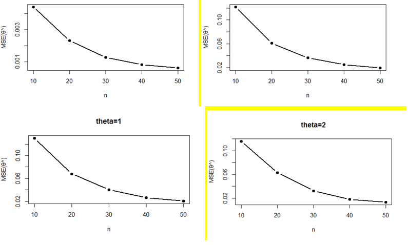
Figure 6 Estimated mean squared error of the MLEs for different values of θ and n.

Data set 1: Present data have been taken from Jones et al.,¹¹ and it is associated with behavioral science. The detailed about data are given in Jones et al.¹¹ A study conducted by the authors in a city located at the south part of Chile has allowed collecting real data corresponding to the scores of the GRASP scale of children with frequency in parenthesis, which are:

19(16)    20(15)   21(14) 22(9)        23(12)   24(10)   25(6) 26(9)           27(8)     28(5)     29(6)      30(4)      31(3)     32(4) 33 34          35(4)      36(2)     37(2) 39                42 44

Data set 2: This data set is the strength data of glass of the aircraft window reported by:¹²
18.83      20.8     21.657   23.03      23.23      24.05      24.321   25.5      25.52      25.8        26.69     26.77   26.78    27.05      27.67      29.9      31.11     33.2        33.73      33.76     33.89   34.76    35.75      35.91      36.98     37.08    37.09          39.58      44.045   45.29    45.381

Data Set 3: The following data represent the tensile strength, measured in GPa, of 69 carbon fibers tested under tension at gauge lengths of 20mm taken from.¹³

 1.312     1.314      1.479      1.552      1.700      1.803      1.861      1.865      1.944      1.958      1.966      1.997      2.006      2.021      2.027      2.055      2.063      2.098      2.140      2.179      2.224      2.240      2.253      2.270      2.272      2.274      2.301      2.301      2.359      2.382      2.382      2.426      2.434      2.435      2.478      2.490      2.511      2.514      2.535      2.554      2.566      2.570      2.586      2.629      2.633      2.642      2.648      2.684      2.697      2.726      2.770      2.773      2.800      2.809      2.818      2.821      2.848      2.880      2.954      3.012      3.067      3.084      3.090      3.096      3.128      3.233      3.433      3.585      3.858     

From Above data sets, Pranav distribution has been fitted along with one parameter Sujatha, Ishita and and Akash, Shanker ,Lindley and exponential distributions. pdf, and cdf of these distributions are given in Table 2. The ML estimates, values of$-2\ln L$ and K–S statistics of the fitted distributions are shown in Table 3.

Profile plots of MLE of parameter and fitted probability plots of proposed distributions, on considered data sets are given in the Figure 7–9 respectively.

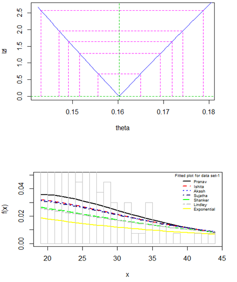
Figure 7 Profile plot of parameter and fitted probability plot of distributions for dataset-1.

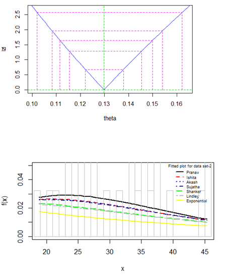
Figure 8 Profile plot of parameter and fitted probability plot of distributions for dataset-2.

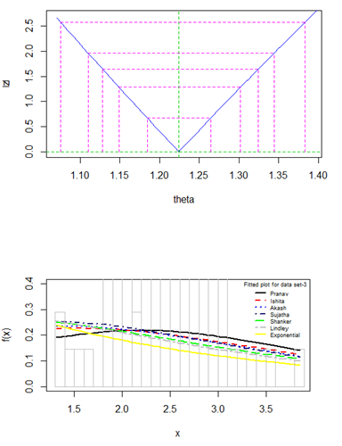
Figure 9 Profile plot of parameter and fitted probability plot of distributions for dataset-3.

In this study, a new one parameter Pranav distribution has been proposed. Its mathematical properties including moments, coefficient of variation, skewness, kurtosis, index of dispersion, hazard rate function, mean residual life function, stochastic ordering, mean deviations, order statistics, Bonferroni and Lorenz curves, and stress–strength reliability have been discussed. Simulation study of Pranav distribution has also been discussed. The method of moments and the method of maximum likelihood estimation have been derived for estimating the parameter. Finally, three numerical examples of real lifetime datasets form Biology have been presented to test the goodness of fit of the Pranav distribution. Its fit was found satisfactory over exponential, Lindley, Sujatha, Ishita, Akash and Shanker distributions. It can be considered as good model for biological study.

Note: The paper is named Pranav distribution in the name of my eldest son Pranav Shukla.

None.

Author declares that there is no conflict of interest.

1. Lindley DV. Fiducial distributions and Bayes’ theorem. Journal of the Royal Statistical Society, Series B. 1958;20(1):102–107.
2. Shanker R. Akash distribution and Its Applications. International Journal of Probability and Statistics. 2015;4(3):65–75.
3. Shanker R. Shanker distribution and Its Applications. International Journal of Statistics and Applications. 2015;5(6):338–348.
4. Shanker R, Shukla KK. Ishita distribution and Its Applications. BBIJ. 2017;5(2):1–9.
5. Shanker R. Sujatha Distribution and Its Applications. Statistics in Transition–New series. 2016;17(3):1–20.
6. Ghitany ME, Atieh B, Nadarajah S. Lindley distribution and its Applications. Mathematics Computing and Simulation. 2008;78:493–506.
7. Shaked M, Shanthikumar JG. Stochastic Orders and Their Applications. New York: Academic Press; 1994.
8. Bonferroni CE. Elementi di Statistca generale, Seeber, Firenze; 1930.
9. Renyi entropy. On measures of entropy and information. Proc Fourth Berkeley Symp on Math Statist and Prob. 1961;(1):547–561.
10. Balakrishnan N, Victor L, Antonio S. A mixture model based on Birnhaum–Saunders Distributions. A study conducted by Authors regarding the Scores of the GRASP (General Rating of Affective Symptoms for Preschoolers), in a city located at South Part of the Chile; 2010.
11. Jones O, Maillardet R, Robinson A. Introduction to scientific Programming and Simulation using R. New York: Taylor & Francis Group; 2009.
12. Fuller EJ, Frieman S, Quinn J. Fracture mechanics approach to the design of glass aircraft windows: A case study. SPIE Proc. 1994;(2286):419–430.
13. Bader MG, Priest AM. Statistical aspects of fiber and bundle strength in hybrid composites, In; Hayashi T, Kawata K, Umekawa S, editors. Progress in Science in Engineering Composites, ICCM–IV, Tokyo. 1982:1129–1136.