A numerical model combining Detached Eddy Simulation (DES) and low Mach number preconditioning in an unstructured, adaptive finite volume solver with implicit time discretisation is used for fully turbulent flow simulation over a high-lift configuration. The developed numerical procedure with preconditioning is demonstrated to be computationally efficient in improving the convergence behavior compared to the un-preconditioned scheme. The use of Zonal DES is shown to precisely predict the stall angle compared to the original Reynolds Averaged Navier-Stokes (RANS) model. The above numerical scheme with a multiscale based grid adaptation technique to capture the detailed flow features over the high-lift configuration demonstrates the computational efficiency and reliability of the developed model. The results are compared with the experimental data available in the existing literature.

Keywords: Detached Eddy Simulation, DES, Low Mach number preconditioning, Implicit scheme, High-Lift configuration, Adaptive turbulent simulation, Stall inception

$Q$ Flow vector with conservative variables

$Q_L$  Conservative vector at the grid level L

$Q_{{}_{{}_{{}_l}}}$  Left hand state conservative flow vector

$Q_r$  Right hand state conservative flow vector

$\Delta \Omega$  Control volume

Res Total residual

${\mathrm{Res}}_c$  Convective component of residual

${\mathrm{Res}}_{{}_v}$  Laminar viscous component of residual

${\mathrm{Res}}_{{}_t}$  Turbulent viscous component of residual

$W$  Flow vector with primitive variables

$F$  Conservative flux vector

$J$  Jacobian matrix

$\Delta t$  Timestep

$ds$  Elemental surface area

$\Delta S_i$  Discrete elemental surface quadrature for flux estimation

$n$  Normal vector to control volume surface area

$\rho$  Density

$u,v,w$  Component of the velocity vector along the Cartesian direction

$\tilde{V}$  Turbulent transport variable in Spalart-Allmaras model

$T$  Static temperature

$M$  Mach number

$M_{\infty }$ > Free stream Mach number

$M_n$  Mach number normal to the face

$a$  Sound speed

$R$  Gas constant

$C_p$  Specific heat at constant pressure

$H$  Total enthalpy              

$V_n$  Normal velocity used in low Mach number preconditioning

$U_r$  Reference velocity for low Mach number preconditioning

$M_r$ Reference Mach number for low Mach number preconditioning

$K$  Cut-off parameter for the preconditioning (set to 0.5)

${\Gamma }_c,{\Gamma }_v$  Preconditioning matrix in conservative and primitive forms

$\in$  Cut-off parameter in preconditioned scheme

$\Delta r$  Grid characteristic length for preconditioning

$\Delta x,\Delta y$  Maximum and minmum dimension of the grid cell

$v$  Laminar kinematic viscosity

$C_p$  Surface static pressure coefficient

$C_l$  Lift coefficient

$C_d$  Drag coefficient

$\lambda$  Eigenvalues of the Jacobian matrix

$d_w$  Wall distance

$C$  Chord length

$\alpha$  Angle of attack

Superscripts

$n$  Iteration loop

SFB, Sonder Forschung Sbereich; RANS, Reynolds Averaged Navier-Stokes Equation; MUSCL, Monotonic Upwind Scheme For Conservation Laws

Aerodynamic design of a multi-element high-lift configuration is an integral part of the overall wing design process. The configuration is comprised of slat, main element, flap;¹ and is operational during take-off as well as landing phases of the aircraft in the flight envelop. Evaluating aerodynamic parameters of such configuration in the form of lift and drag coefficients in a rapid design loop for shape optimization relies heavily on the computational efficiency and reliability of the underlying flow solver. This effort is challenging; i) because of the requirements to capture complex interaction of the flow structures determining the physical phenomenon; ii) the numerical model should be computationally efficient and accurate enough to predict the physics reliably. Resolution of the flow structures and reliable prediction of the aerodynamic performance over such a configuration poses significant numerical challenges due to the nature of the flow field with the presence of mutually interacting shear layer from the upstream components with the boundary layers developed in the downstream regions, fluid undergoing high acceleration on the suction surface of the slat to create a localized supersonic patch in a predominantly low speed flow and the presence of vortices in the inter-element gaps. Comparatively lower free stream Mach number corresponding to the take-off/landing conditions creates a flow with varying compressibility where a small region of transonic flow domain is surrounded by a large region of low speed flow. The complexity of the flow phenomenon with multiple physical mechanisms surrounding the high-lift configuration is explained by AMO Smith.²

The enormity of the task can be gauged from several research programs being conducted in the past and currently being running; e.g. HIRENASD,³ AST/IWD,⁴ EUROLIFT,⁵ MEGAFLOW.⁶ Several studies have been conducted on flow simulation, analysis and design of high lift configuration; e.g. Aerodynamic Shape Optimization using a viscous adjoint method,⁷ delaying flow separation on the flap surface by periodic injection of air,⁸ numerical modelling of transition⁹ and aerodynamic simulation.¹⁰ Requirements of using highly stretched boundary layer grid to resolve the near wall flow at high Reynolds number, large scale variation in flow compressibility due to the change in local Mach number, localized presence of shock and vortical flow structures as well as most critically, the inability to predict inception of flow separation using a RANS model have been discussed. The current paper describes an improved numerical model to resolve the above described flow phenomenon with accuracy and speed. Low Mach number preconditioning is used to speed up the simulation time. A Zonal DES (Detached Eddy Simulation) proposed^11,12 is applied to improve the prediction of the baseline RANS turbulence model; especially near stall. The computational efficiency of the solver is achieved through a grid adaptation method, tightly integrated to the solver and grid generation modules to selectively refine the mesh in the required regions to capture the flow field while restricting the requirement to significantly increase the mesh count. In this work, we combine the use of low speed preconditioning with grid adaptation and Zonal DES model to capture the flow field reliably to predict the stall inception angle with reduced computational effort. The paper is organized as follow. The section on Numerical Method provides a brief introduction of the schemes in the baseline solver. The implementation and validation of preconditioning technique and the Zonal DES methods are described in detail; followed by the section on Results and Discussion.

The geometry used in this work is a multi-element high-lift profile BAC3-11/RES/30/21; defined as the reference configuration in the Collaborative Research Program (SFB401). It comprises of an upstream slat, the main element and a downstream single slotted flap with geometrical dimensions as described in the report by Moir.¹ The slat and flap are deflected at 25° and 20°; respectively.

Baseline Solver

A CFD software package Quadflow, developed within the Collaborative Research Program, “Flow Modulation and Fluid-Structure Interaction at Airplane Wings” is used as the baseline solver. The package is comprised of tightly integrated three modules; a multi-block structured mesh generator, Multiscale based grid adaptation and an unstructured implicit, cell centered, finite volume RANS solver; for detail, see chapter2, Schroeder W et al.¹³

The grid generator parametrically transforms the CAD geometry in the physical domain to the logical computational space. In order to avoid the loss of geometrical information, B-Spline is used for mapping. Each cell in the final multi-block structured mesh is represented with block, level and index (i,j for 2D) information for multiscale analysis. The grid interfaces at the block boundaries are non-matching (Figure 1).

Figure 1 Grid generation and adaptation techniques in Quadflow.

Parametric surface mapping Pyramid scheme of multiscale transformation

The grid adaptation is carried out using multiscale decomposition; which divides the solution variables at the cell center into a sequence of cell averages (Q_L-1) and the detail coefficients (d_L-1). The amount of variation in the detail coefficient guides the grid adaptation; which not only refines but also coarsens the mesh in the computational domain during flow resolution. Number of refinement levels and its intensity are controlled by user specified parameters. For detail on the grid generation and grid adaptation, refer.^14,15

The implicit solver¹⁶ uses backward-Euler for time discretization.

$\Delta Q^n=-J^{-1}\mathrm{Re}s\left(Q^n\right)$ (Eqn. 1)

Where the flux Jacobian is defined as

$J=\left[{\Gamma }_c\frac{I}{\Delta t}\Omega +\frac{\partial }{\partial Q}Res\left(Q^n\right)\right]$ (Eqn. 2)

and constructed analytically using ADIFOR.¹⁷

The total residual is the contribution from convective, laminar viscous and turbulence fluxes.

$Res(Q^n)=Re{s}_c(Q^n)+Re{s}_v(Q^n)+?Re{s}_t(Q^n)$ (Eqn. 3)

Convective contribution to the residual is estimated by integrating the interface fluxes evaluated using an approximate Riemann solver, HLLC¹⁸ at the Gauss Quadrature of the interface. The left and right hand state variables at the interface are reconstructed using the gradients at the cell centers from the cell averaged values and limited to eliminate any newly developed maxima or minima according to the TVD condition for non-linear stability. Green-Gauss integral formulation is used for computing gradients at the cell centers and Venktakrishan’s formulation¹⁹ is used for enforcing TVD condition. The scheme is based on MUSCL with second order spatial accuracy in the numerical model.

$Re{s}_c\left(Q^n\right)={{\displaystyle {\displaystyle \oint }}}^{\text{}}F\left(Q_l,Q_r\right).n ds={\displaystyle {\sum }_{i=1}^N}{F}_n\left(Q_l,Q_r\right)\Delta S_i$ (Eqn. 4)

The numerical formulation also includes the contribution from laminar viscous fluxes with central discretisation and includes gradient correction as suggested by Weiss.²⁰ One equation Spalart-Allmaras RANS model²¹ is used for turbulence modelling. The system of linear equations at each timestep from the Newton linearization of the above model is solved using pre-conditioned GMRES through PetSC.²² Use of implicit scheme in the above model relaxes the CFL condition and with the highly stretched grid for RANS simulation on the high-lift configuration, a maximum CFL number of 50 is used. The CFL number starts with a smaller value and ramps up as the iteration proceeds.

Initial computation starts with a coarse mesh and as the residual converges to a certain level (pre-specified by the user; for these cases under consideration the drop is of the order of 6); the multiscale analysis is carried out resulting in a locally refined grid depending on the flow field. The simulation continues with the refined grid till a grid independent lift and drag coefficients are obtained.

The sequence of steps in computation with grid adaptation using implicit time integration scheme is shown in the flowchart (Figure 2).

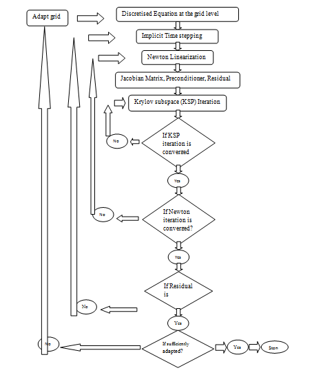
Figure 2 Solution process with grid adaptation using implicit scheme.

Low Mach number preconditioning

Numerically, Navier-Stokes equations solved using time marching scheme exhibit hyperbolic nature and the characteristic variables are propagated at speeds, detected by the eigenvalues of the Jacobian matrix. At a lower Mach number, the disparity between the faster acoustic wave (at sonic speed) and slower material wave (moving at the flow speed) results in a high condition number (Ratio of the maximum to minimum eigenvalues) of the Jacobian matrix that imparts stiffness to the numerical scheme. Chorin²³ used artificial compressibility to scale the time varying pressure term; thus artificially modifying the acoustic speed to bring the condition number down for extending the validity of the time marching approach for incompressible flow conditions. Changing the time derivative term in the governing equation doesn’t impact the accuracy of the steady state solution. The approach proposed by Chorin and its subsequent extension by Radespiel et al.,²⁴ Weiss & Smith,²⁵ Darmofal²⁶ led to the development of low Mach number preconditioning approach in the framework of density based method for effective flow simulation at lower Mach number.

In this work, the preconditioning matrix for the primitive variables proposed by Weiss and Smith²⁵ is used and the method is shown to be effective for a flow region with a mixture of compressible and incompressible flow fields.

${\text{Γ}}_p=\lfloor \begin{array}{l}\left({\theta }_p+\raisebox{1ex}{$1$}\!\left/ \!\raisebox{-1ex}{$RT$}\right.\right) 0 0 0 \raisebox{1ex}{$-\rho $}\!\left/ \!\raisebox{-1ex}{$T$}\right. 0 \\ \left({\theta }_p+\raisebox{1ex}{$1$}\!\left/ \!\raisebox{-1ex}{$RT$}\right.\right) \rho 0 0 \raisebox{1ex}{$ -\rho u$}\!\left/ \!\raisebox{-1ex}{$T$}\right. 0\\ \left({\theta }_p+\raisebox{1ex}{$1$}\!\left/ \!\raisebox{-1ex}{$RT$}\right.\right)v 0 \rho 0 \raisebox{1ex}{$ -\rho v$}\!\left/ \!\raisebox{-1ex}{$T$}\right. 0\\ \left({\theta }_p+\raisebox{1ex}{$1$}\!\left/ \!\raisebox{-1ex}{$RT$}\right.\right)w 0 0 \rho \raisebox{1ex}{$ -\rho w$}\!\left/ \!\raisebox{-1ex}{$T$}\right. 0\\ \left({\theta }_p+\raisebox{1ex}{$1$}\!\left/ \!\raisebox{-1ex}{$RT$}\right.\right)H-1 \rho u \rho v \rho w \raisebox{1ex}{$ \rho (C_p-H$}\!\left/ \!\raisebox{-1ex}{$T$}\right.) 0\\ \left({\theta }_p+\raisebox{1ex}{$1$}\!\left/ \!\raisebox{-1ex}{$RT$}\right.\right)\tilde{V} 0 0 0 \rho \rho \end{array}\rfloor$ (Eqn. 5)

As Quadflow uses solution variables in conservative form at the cell center, the preconditioning matrix is transformed from primitive variable to conservative form. $\frac{\partial W}{\partial Q}$ is the transformation matrix in Eqn. (6).

${\text{Γ}}_c={\text{Γ}}_p\frac{\partial W}{\partial Q}$ (Eqn. 6)

The resulting preconditioning matrix pre-multiplies the block Jacobian matrix that constitutes global Jacoabian matrix for the system of linear equation, as shown in Eqn. (2).

Comparison of the condition number between pre-conditioned and un-preconditioned schemes (Figure 3) shows, the scaling with the preconditioning matrix limits the condition number to become very large within the incompressible flow regime (local Mach number <=0.3) and thus relieves the original un-preconditioned scheme from its inherent numerical stiffness.

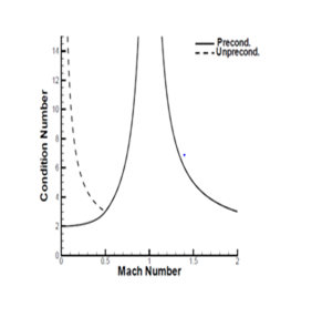
Figure 3 Comparison of condition number.

The preconditioning parameter in preconditioning matrix is, ${\text{θ}}_{\text{p}}=\frac{1}{{\text{u}}_{\text{r}}^2}-\frac{1}{{\text{a}}^2}$ ; (Eqn. 7);

and the reference speed is estimated by, ${\text{u}}_{\text{r}}={\text{M}}_{\text{r}}\text{a}$ . The reference Mach number depends on a cut-off parameter (ε), local Mach number normal to the face and is defined as,

$M_r=\{\begin{array}{l}\epsilon \\ \sqrt{(\frac{2.0M_n^2}{1-2.0M_n^2})}\\ 1\end{array}$ $\begin{array}{l}if Mn\le \epsilon ;\\ if Mn\in (\epsilon ,0.5);\\ if Mn>\mathrm{0.5.}\end{array}$ (Eqn 8)

As the local Mach number of the flow reaches above 0.5, the reference Mach number becomes unit and the preconditioned scheme reverts back to original un-preconditioned formulation.

The cut-off parameter (ε) controls the formulation near stagnation region where the local Mach number reaches close to zero. It is expressed as a function of free stream Mach number for the inviscid flow. For viscous flow (both laminar and turbulent) simulations, diffusive Mach number is used to limit the maximum cut-off value. The diffusive Mach number is ratio between cell Reynolds number and local sound speed.

$\epsilon =\max (K*M_{\infty },\frac{U\Delta r}{ua})$ (Eqn. 9)

In order to estimate the diffusive Mach number, a characteristic length scale based on the grid size is required. “Δr” is the characteristic length used in the formulation. It is a function of local grid size and is defined as

$\Delta r=\frac{\Delta x\Delta y}{\sqrt{{\left(\Delta x\right)}^2+{\left(\Delta y\right)}^2}}$ (Eqn. 10)

The modified eigenvalues of the preconditioned system are used as the replacement of the original wave speeds in the HLLC approximate Riemann solver.¹⁸ The wave speeds of the preconditioned equation is

$\lambda ({\Gamma }_c^{-1}\frac{\partial F}{\partial x})=\frac{1}{2}(1+M_r^2)V_n\pm \frac{a}{2}\sqrt{{(\_1-M_r^2)}^2{M}_n^2+4M_r^2},V_n$ (Eqn. 11)

In order to extend a base solver with implicit time integration for low speed preconditioning, changes are required to i) Include the preconditioning matrix to modify the Jacobian term, ii) Replace the wave speeds of Riemann solver with the preconditioned eigenvalues and iii) change the timestep with maximum eigen value of the preconditioned formulation.

Zonal DES

Turbulence modelling using RANS approach targets to model all the spatial turbulent scales in the flow domain and doesn’t consider the grid resolved components that are already captured in the mean quantities. Thus, RANS is a reliable model as long as the fluctuating turbulence quantities remain smaller compared to the grid size. As the flow tends to separate, the turbulent eddies become larger; thus a part of the contribution from the turbulence is captured as the averaged flow quantities through grid. Using eddy viscosity model to correlate the Reynolds stress with the above increased averaged flow quantities leads to a dual inclusion of the turbulence; causing an over-prediction of turbulence in the flow. Increased turbulence in the flow results in delayed separation which is commonly observed in analysis using RANS model.¹⁰

This drawback of RANS imposing a limitation on accurately resolving and modelling the turbulence scales in the region of separated flow field has been reported by Franke et al.²⁷ To enhance the applicability of RANS model, Rung²⁸ suggested the ratio between the grid resolved timescale and modelled turbulent timescale to satisfy a condition based on Reynolds and Stanton number. Another approach as suggested by Spalart to use RANS formulation in the boundary layer flow at the near wall region while using LES model at far away distance. This is achieved by re-defining the wall distance as proposed by Ref²⁹ in the original Spalart-Allmaras model in a selected region to modify the destruction term to limit the net turbulence generation. This above modification is applied at the regions far away from the viscous wall; terms as LES type region of DES model and separated from the near wall RANS region.

A boundary in percentage of chord length separating the near wall region from the LES domain is specified a priori, thus making it equivalent to Zonal DES.³⁰ The effect of dimension of the specified boundary to separate the RANS and LES regions on the accuracy of the solution is evaluated during validation of the method and provided in the Results section. In order the model to provide accurate result, the grid requires to have high aspect ratio cells near the boundary and isotropic cells in the far away region; which is automatically achieved in the current work using grid adaptation.

Wall distance plays a critical role in transforming RANS formulation to DES. Additionally, its method of estimation plays a crucial role in controlling the accuracy of the solver; especially in the presence of grid adaptation, as explained follow. Refinement of the boundary layer in a grid adaptive solver leads to the presence of highly stretched cells near the wall. Using a commonly adopted approach to compute the wall distance by estimating the distance between surface wall nodes from the cell center leads to inaccurate estimation of wall distance. In order to alleviate the problem, the wall distance is estimated using vector algebra.

The distance of a point on the surface from the cell center is expressed in a parametric form and the distance is minimum for a specific value of the parameter (t). Wall distance is estimated from the cell center to the point on the surface with the minimum distance.

And the distance is minimum when, $\begin{array}{l}r=r_1+t{r}_2,\\ |r{|}^2=(r_1^2+t^2{r}_2^2+2t{r}_1.r_2)\end{array}$ (Eqn. 12)

The above estimated wall distance is subsequently modified with the condition below to achieve Zonal DES.

$d_w=\{\begin{array}{l}Unchanged d_w\le 0.1\times C\\ 0.65\times \max (\Delta x,\Delta y) d_w>0.1\times C\end{array}$ (Eqn. 13)

The wall distance is unchanged if it is lower than 0.1 of the chord length; which represents the cells within the boundary layer and the intention is to activate the RANS model in the region. Away from the profile surface, the wall distance is estimated using the grid dimension; resulting in lower wall distance. This change increases the destruction term in the turbulence model and reduces the eddy viscosity (Figure 4).

Figure 4 Method of wall distance estimation, a typical adapted grid near boundary layer, Zonal DES.

Wall distance estimation Stretched cells in refined boundary layer Zonal DES boundary

To validate the implemented formulation on preconditioning, fully turbulent flow computation is performed over RAE2822 profile at free stream Mach number, =0.01, angle of attack, α=1.89° and Reynolds number, Re=5.7E6. The initial grid has 400 cells and the final solution is obtained after three levels of grid adaptation with the computational domain comprising of 14,899 cells (Figure 5).

Figure 5 Adapted grid and turbulent flow simulation over RAE2822 at ${\text{M}}_{\infty }$ =0.01.

 Final level adapted grid Mach no. variation in the domain Surface pressure coefficient

Surface distribution of  value below unit is achieved in the finest grid level. As expected, relatively lower value of the Mach number restricts the grid adaptation within the boundary layer; which is the highest active region in the computational domain. The surface distribution of the static pressure coefficient on the final level grid is compared with the computationally estimated data by Radespiel.²⁴ In the current simulation, the flow is assumed to be fully turbulent, whereas the case available in the literature; the flow is tripped to turbulent at 11% chord length from the leading edge. Hence, skin friction coefficient is not compared.

Validation of Zonal DES Method

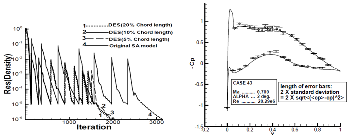
To validate the Zonal DES model and the effect of pre-defining the boundary to separate RANS and LES like zone on the solution; the simulation is carried out on the cruise configuration of the BAC 3-11/RES/30/21 profile. The results from the numerical simulations are compared with the available data from the experiment carried out at KRG cryogenic wind tunnel at DLR Goettingen.³¹

The operating point for the simulation corresponds to the Case43 of the KRG experimental data; with free stream Mach number=0.7, angle of attack=2.0° and Reynolds number=20.29E6 (Figure 6).

Figure 6 Initial coarse mesh and final adapted meshes at two simulation.

Comparison of convergence at different DES boundary Comparison of surface $C_p$ with experimental data

Three different values of the zonal boundaries are specified with respect to the chord length. Comparison of the number of iterations to achieve the convergence and surface static pressure distribution show a minor effect of the distance used to separate out RANS from LES like zone on the flow solution.

Application on the high-lift configuration

The implicit adaptive solver with above described implementation of low Mach number preconditioning and Zonal DES is applied to simulate the flow field over the high-lift configuration. The initial H grid has 61 blocks with 16740 quadrilateral cells. At the coarsest grid level, the airfoil surface boundary has 408 elements with a maximum y+ of 30. The grid is extended to 25 chords along the upstream and downstream directions to reduce the effect of wakes on the far field boundary. The free stream Mach number is 0.197 and Reynolds number based on the chord length is 3.52million. Two simulations are performed at angle of attack 4.01° and 20.18°. Comparison of the initial coarse mesh with the final mesh after six levels of adaptation is shown in Figure 7.

Figure 7 Initial coarse mesh and final adapted meshes at two simulations.

 Initial coarse grid Final grid, 6 adaptation (α=4.01⁰) Final grid, 6 adaptation (α=20.18⁰)

The adaptation module can detect the regions of high variation in flow, e.g. boundary layer, wakes in the flow field, vortex in the inter-elemental gap and the mesh is automatically refined. The final computational domain contains approximately 180,000 cells with 1900 cells on the airfoil surface. A rapid change in the number of cells in the computational domain is observed during initial phase of grid adaptation as the solution undergoes significant change due to the developing flow structures. In the later phase of grid adaptation, the variation of cell number in the domain is decreased. Refinement of the cells in the boundary layer during grid adaptation reduces the y+ value on the airfoil surface and at the finest level the y+ value below unit is achieved.

Details of the flow field, surface pressure coefficient variation and the Mach number distribution for the two simulations are shown in Figure 8. Comparison of the surface pressure coefficient from the numerical results with the available experimental data¹ shows a close agreement.

 Close up view of adapted grid Mach number variation at α=4.01⁰ Comparison of $C_p$ at α=4.01⁰

Figure 8 Adapted grids, Mach number variation and $C_p$ variations for two simulations.

Adapted grid in inter-element gaps Mach number variation at α=20.18⁰ Comparison of $C_p$ at α=20.18⁰

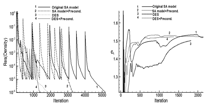
Three sets of additional simulations are performed at an angle of attack set to 4.01° with original Spalart-Allmaras model, Original SA model with Preconditioning, Detached Eddy Simulation (DES) to compare the convergence behavior and accuracy of the results. The original SA model takes more number of iterations to achieve the required residual drop and developing the lift coefficient as evident in Figure 9. Contrastingly, the required number of iterations is around 3.7times lower with DES+preconditioning and the aerodynamic parameter achieves stability much ahead of the un-preconditioned simulation. Interestingly, though DES without preconditioning converged faster (as shown in the residual drop); but the lift coefficient is still under evolution.

Figure 9 Initial coarse mesh and final adapted meshes at two simulation.

Comparison of the residual drop Comparison of the evolving lift coefficients

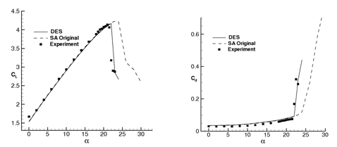
Following investigation is carried out to compare the ability of the developed model in accurately predicting the stall angle compared to the original RANS formulation. Simulations are carried out on the high lift configuration using original SA and the newly developed DES model at multiple angles of attack ranging between 0° to 30° in steps of 2° with steady time integration scheme (Figure 10).

Figure10 Comparison of the estimated aerodynamic performance.

Comparison of the $C_L$ $C_d$ ~ angle of attack Comparison of the  ~ angle of attack

The grid is refined successively during adaptation depending on the flow field which is eventually determined by the angle of attack. As expected, the lift coefficient increases linearly with the angle of attack till stall occurs. At the stall condition, the computation is characterized by non-convergence of the residual (despite steady time integration scheme is used) as shown in Figure 11. The difference is the original SA model predicts the non-convergence at α=26°, whereas the DES model with preconditioning exhibits the same behavior at α=23°.

Figure11 Comparison of drop in residual at different angles of attack (Steady state simulation).

Computation using original SA model Computation using DES+Preconditioning model

Any subsequent increase in the angle of attack shows an oscillatory behavior in the residual with no converged results. The non-convergence of the flow field is also illustrated by a corresponding fluctuation of the lift coefficient about a mean value (not shown in the paper).

To confirm the unsteady nature of the flow field accurately, the simulation is carried out in time accurate manner using a second order time accurate Backward difference scheme with DES and Preconditioning model. The angle of attack is set to 23°. The criterion for grid adaptation is changed to activate the refinement after every timestep rather than the depending on the drop-in convergence. Figure 12 shows the oscillatory nature of the lift coefficient and vortices in the separated flow regions.

After confirmation of the unsteady nature of the flow field, the lift and drag coefficients at the sequence of angle of attacks from both the models are compared with the experimental data (Figure 10). The plot shows the stall angle predicted by the DES with preconditioning matches well with the experiment compared to the results from the original SA model; where the stall inception angle is over-predicted.

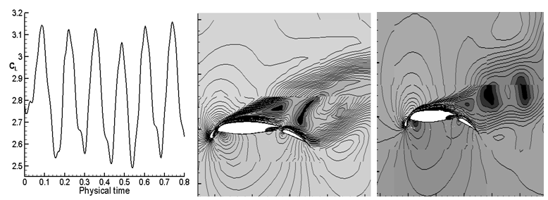
Figure 12 Unsteady simulation using DES with preconditioning at 23⁰ .

$C_L$ showing unsteadiness at α=23⁰ Flow field showing separated flow region at α=23⁰

In the current work, a numerical model is developed by combining low Mach number preconditioning with DES in an implicit, unstructured, finite volume adaptive solver to simulate the flow fields over high lift configuration. Formulation, implementation of the above methods and their physical relevance is explained. The combination of the low Mach number preconditioning and Zonal DES formulations in the grid adaptive implicit solver is demonstrated to provide approximately 4times speed up while accurately capturing the stall inception angle. The improvement in computational efficiency provided by the scheme depends on the amount of low speed flow region in the computational domain and is effective in the presence of varying flow compressibility; even when a small supersonic patch appears in the flow field. Secondly, the agreement of predicted lift coefficient and surface pressure coefficient distribution with the experimental data confirms the accuracy of the developed numerical model. The non-convergence of steady time integration scheme and the subsequent confirmation of the unsteady flow field with the unsteady time integration scheme at the stall inception demonstrate the effectiveness of the DES model to predict stall compared to the original RANS formulation.

None.

The author declares that there is no conflict of interest.

1. Moir IRM. Measurements on a Two-Dimensional Aerofoil with High-Lift Devices. AGARD-AR-303: A Selection of Experimental Test Cases for the Validation of CFD Codes. 1994:1&2.
2. Smith AMO. High-Lift Aerodynamics. Journal of Aircraft. 1975;12(6):501–530.
3. Ballmann J, Dafnis A, Braun C, et al. The HIRENASD Project: High Reynolds number Aerostructural Dynamics Experiments in the European Transonic Windtunnel (ETW). ICAS 2006, 25^th International Congress of the Aeronautical Sciences, 2006.
4. Slotnick JP, et al. Navier-Stokes Analysis of a High Wing Transport High-Lift Configuration with Externally Blown Flaps. AIAA-2000-4219, 18^th AIAA Applied Aerodynamics Conference, Denver/Colorado; 2000.
5. European High Lift Programme II (2007), EADS Airbus Gmbh(D), EADS Airbus SA(F), EADS CASA(E), ALENIA(I), Dassault Aviation(F), ETW Gmbh(D), DLR(D), ONERA(F), CIRA(I), NLR(NL), FOI(S), INTA(E), IBK(D), ASR(EL).
6. Rudnik R, Melber S, Ronzheimer A, et al. Three-Dimensional Navier-Stokes Simulations for Transport Aircraft High-Lift Configurations. Journal of Aircraft. 2001;38(5):895–903.
7. Kim S, Alonso JJ, Jameson A. Design Optimisation of High-Lift Configurations Using a Viscous Continuous Adjoint Method. AIAA 2002-0844, 40th AIAA Aerospace Sciences Meeting and Exhibit, Reno/NV; 2002.
8. Schatz M, Thiele F. Numerical Study of High-Lift Flow with Separation Control by Periodic Excitation. AIAA 2001-0296, 39th AIAA Aerospace Sciences Meeting and Exhibit, Reno/NV; 2001.
9. Krumbein A. Automatic transition prediction and application to high-lift multi-element configurations. Journal of Aircraft. 2005;42(5):1150–1164.
10. Rudnik R, Melber S, Ronzheimer A, et al. Three-Dimensional Navier-Stokes Simulations for Transport Aircraft High-Lift Configurations. Journal of Aircraft. 2001;38(5):895–903.
11. Soda A, Knopp T, Weinham K. Numerical Investigation of Transonic Shock Oscillations on Stationary Aerofoils. Symposium on Hybrid RANS-LES Methods Stockholm, Sweden; 2005.
12. Spalart P. Strategies for turbulence modelling and simulations. International Journal of Heat and Fluid Flow. 2000;21(3):252–263.
13. Schroeder W, et al. Summary of Flow Modulation and Fluid-Structure Interaction Findings. Notes on Numerical Fluid Mechanics and Multidisciplinary Design. 2009;109:25–52.
14. Mueller S. Multiscale Schemes for Conservation Laws. Lecture Notes on Computational Science and Engineering. 2002:27.
15. Lamby P. Parametric Multi-Block Grid Generation and Application to Adaptive Flow Simulations. Dissertation, RWTH-Aachen; 2007.
16. Ray SR. Contribution to the Development of an Adaptive solver for Numerical Simulation of Steady and Unsteady Flows. PhD Thesis, RWTH Aachen, 2013.
17. Bischof C, Carle A, Hovland P, et al. ADIFOR 2.0 Users' Guide, Mathematics and Computer Science Division. Center for Research on Parallel Computation, Technical Report CRPC-95516-S, 1998.
18. Batten P, Clarke N, Lambert C, et al. On the Choice of Wave Speeds for the HLLC Riemann Solver. Siam Journal of Scientific Computing. 1997;18(6):1553–1570.
19. Venkatakrishnan V. Convergence to steady state solutions of the Euler equations on unstructured grids with limiters. Journal of Computational Physics. 1995;118(1):120–130.
20. Weiss JM, Maruszewski JP, Wayne AS. Implicit Solution of the Navier-Stokes Equation on Unstructured Meshes. AIAA 97-2103, 1997.
21. Spalart P, Allmaras S. A One-Equation Turbulence Model for Aerodynamic Flows. AIAA 92-0439, 1992.
22. Balay S, et al. PETSc Users Manual, ANL-95/11 - Revision 2.1.5. Argonne National Laboratory, 2004.
23. Chorin AJ. A numerical method for solving compressible viscous flow problems. Journal of Computational Physics. 1967;2(1):12–26.
24. Radespiel R, Turkel E, Kroll N. Assessment of Preconditioning Methods. Forschungsbericht 95-29. Braunschweig: Institut fuer Entwurfsaerodynamik; 1995.
25. Weiss JM, Smith WA. Preconditioning Applied to Variable and Constant Density Flows. AIAA Journal. 1995;33(11):2050–2057.
26. Darmofal DL, Van Leer B. Local Preconditioning of the Euler Equations: A Characteristic Interpretation. 30^th Computational Fluid Dynamics, VKI Lecture Series. 1999:1.
27. Franke M, Rung T, Schatz M, et al. Numerical simulation of high-lift flows employing improved turbulence modelling. Barcelona: ECCOMAS; 2000.
28. Rung T, Thiele F. Computational modelling of complex boundary-layer flows. Singapore: Int Symp on Transport Phenomena in Thermal-Fluid Engineering; 1996.
29. Spalart P. Young-Person's Guide to Detached-Eddy Simulation Grids. NASA/CR-2001-211032, 2001.
30. Deck Sebastien. Numerical Simulation of Transonic Buffet over a Supercritical Airfoil. AIAA Journal. 2005;43(7):1556–1566.
31. Ballmann J, et al. Experimental Analysis of High Reynolds Number Aero-Structural Dynamics in ETW. 46th AIAA Aerospace Sciences Meeting and Exhibit, Reno, Nevada; 2008.