Submit manuscript...
eISSN: 2574-8092

International Robotics & Automation Journal

Research Article Volume 2 Issue 2

A GPU-based evolution algorithm for motion planning of a redundant robot

Chih Jer Lin, Chin Sheng Chen, Shen Kai Yu

Institute of Automation Technology, National Taipei University of Technology, Taiwan

Correspondence: Chih Jer Lina, Institute of Automation Technology, National Taipei University of Technology, Taiwan, Tel 886-2-2771-2171, Fax 886-2-2711-1401

Received: March 18, 2017 | Published: April 17, 2017

Citation: Lin CJ, Chen CS, Yu SK. A GPU-based evolution algorithm for motion planning of a redundant robot. Int Rob Auto J. 2017;2(2):45-57. DOI: 10.15406/iratj.2017.02.00015

Download PDF

Abstract

Kinematic redundancies of robotic manipulator provide many benefits for motion planning, such as collision avoidance, improved manipulability, flexibility, and singularity avoidance. Based on the task priority, the motion planning of a redundant robot involves solving the associated optimization problem according to the desired criterion. Several kinematic techniques for redundant manipulators have been proposed. However, the computing time of solving the optimization problem with multiple optimization objectives is too large to implement the motion planning in real-time. Therefore, more efficient optimization algorithms are needed for motion planning of redundant robots. This paper presents a new technique to solve the inverse kinematics of redundant manipulators using a GPU-based evolution algorithm. This algorithm combines the optimal perturbation method with a multi-objective function to solve the obstacle avoidance and trajectory tracking at the same time. Simulations and implementations for a self-design manipulator with eight joints considering the optimization with multi-objectives with obstacle avoidance and trajectory tracking are developed. The results reveal that the proposed evolution algorithm based on compute unified device architecture (CUDA) has the much higher performance than the optimal perturbation method. Simulation results also show that the proposed EAMP is 398 times faster than the perturbation method for this case study. Experimental results using NI Compact RIO® validate the proposed method feasible for real-time motion planning of the redundant robot.

Keywords: redundant robots, motion planning, genetic algorithm, singularity problem, parallel processing, CUDA

Introduction

Nowadays, robot manipulators have become increasingly important for automation, and a lot of researches have been disused and developed, such as painting, welding, machining and handling. Recently, robot manipulators are designed for more difficult and complicated tasks, such as rescuing task, cleaning in harsh environments, and training prosthesis. Therefore, redundant manipulators are needed to handle these complicated tasks. A robot is termed kinematically redundant as it possesses more degrees of freedom (DOF) than the required one to execute a given task. When the manipulator is not fully constrained for the trajectory planning, there are chaotic inner motions with unpredictable arm configuration if kinematic redundancy occurs. Most of the research on kinematic redundancy uses these extra degrees of freedom to deal with other task-priority problems; a functional constraint task is imposed to be satisfied along with the end-effector task; typical constraints include cost energy minimization,1–3 avoidance from obstacles,4–7 improved manipulability,8–9 singularity avoidance,10–12 and repetitive motion with joint-velocity limitations.13,14 In general, an analytical inverse kinematics relationship for redundant robots may not be obtained by a straight forward derivation. A class of techniques for solving the inverse kinematics of the redundant manipulators was suggested using the pseudo inverse of the Jacobian matrix through the rates at which the joints are driven. The pseudo-inverse method is also called the generalized inverse method and it is first introduced to the robot control problem by Whitney.15

The pseudo-inverse of the Jacobian matrix guarantees an optimal reconstruction of the desired end-effector velocity with the minimum-norm joint velocity in the least squares sense. Moreover, Klein et al.16 were the first to observe the other undesirable property of the pseudo-inverse method that the repetitive end-effector motions do not necessarily yield repetitive joint motions. Baillieul17 proposed an extended Jacobian matrix, which is a square matrix contains the additional information to optimize a specified cost function. The algorithms, which are based on the extended Jocobian matrix, have a locally cyclic property. Many researchers have been produced in the last few years in this topic. A large volume of research has been proposed in this topic in the last few years such as the quadratic-programming method, optimal-perturbation method,4 Non-dominated Sorting Genetic Algorithm (NSGA-II) and Differential Evolution (DE) methods,18 a multi-objective genetic algorithm for obstacle avoidance,19 the closed-loop inverse kinematics algorithm with GA (CLGA) method20 and hybrid-motion planning method.21 These constrained optimization problems are very complicated, especially as the robot manipulator has hyper-redundant degrees of freedom. Therefore, how to increase the computation performance is a big challenge for the redundant robots in real-time implementation. To solve singularity of redundant robot with task priority problems, this paper proposed a CUDA evolution algorithm to implement real-time motion planning. Genetic algorithm (GA) is a stochastic optimization method for solving many practical problems in engineering, science and business domains, but its execution time may become a limiting factor for some huge optimization problems. Fortunately, the evolution of natural population is very suitable with a parallel architecture, because the most time-consuming fitness evaluations can be performed independently for each individual in population. There are various types of parallelization in GAs: master-slave models, coarse-grained models, fine-grained models, hierarchical models, island models, and hybrid models. The emergence of many-core architectures for GPGPU provides the opportunity to significantly reduce the runtime of many complicated bioinformatics algorithms, such as Sequence and Genome Analysis.22 Using CUDA supplies the system based on commonly available and inexpensive hardware (CPU and GPUs) with more powerful high-performance computing power, which are generally not provided by conventional general-purpose processors. To obtain the optimal inverse kinematic solution for motion planning of a redundant robot with obstacle avoidance, the computation load is very large if the grid search algorithm is used. The motivation of this work is to use a real-coded genetic algorithm (or called evolutionary algorithm, EA) to replace the grid search algorithm to speed up the computation. Genetic algorithm (GA) is a stochastic optimization technique based on the idea of natural evolution and its search process based on natural selection developed by Holland.23 Nowadays graphic processing units (GPU) is emerging as one of the most powerful parallel processing devices due to increasing requirements for real-time 3D rendering. GPU have evolved into very powerful processors, which are especially well suited to address problems that are expressed as data-parallel computations, and their price remained in the range of consumer market. GPUs are optimized especially for SIMD-type processing with massive parallelism. Additionally, a general-purpose computing on graphics processing units (GPGPU) is the means of using a GPU to perform computation in applications traditionally handled by the central processing unit (CPU). CUDA is the computing engine that is accessible to software developers through variants of industry standard programming languages, such as C with NVIDIA extensions and certain restrictions.24,25 CUDA has been enthusiastically received in the area of scientific research. For implementing the real-time motion planning of redundant robots, a CUDA-based evolution algorithm method is proposed to reduce the computing time and make the real-time computing possible. The paper is organized as follows. Section 2 introduces the inverse kinematics of redundant manipulators and the experimental equipment. Section 3 presents the proposed EAMP based on compute unified device architecture (CUDA) programming to speed up real-time computation performance. Section 4 presents the experimental results for motion planning with obstacle avoidance in a workspace. Finally, Section 5 draws the main conclusions.

Problem formulation

A redundant manipulator possesses more degrees of freedom (DOF) than the required to execute a given task. Consider a redundant robot with n DOF and a vector of joint variables is denoted by q = [ q 1 , q 2 , ... , q n ] T MathType@MTEF@5@5@+= feaagKart1ev2aaatCvAUfeBSjuyZL2yd9gzLbvyNv2CaerbuLwBLn hiov2DGi1BTfMBaeXatLxBI9gBaerbd9wDYLwzYbItLDharqqtubsr 4rNCHbGeaGqiVCI8FfYJH8YrFfeuY=Hhbbf9v8qqaqFr0xc9pk0xbb a9q8WqFfeaY=biLkVcLq=JHqpepeea0=as0Fb9pgeaYRXxe9vr0=vr 0=vqpWqaaeaabiGaciaacaqabeaadaqaaqaaaOqaaKqbakaadghacq GH9aqpdaWadaqaaiaadghadaWgaaqcfasaaiaaigdaaeqaaKqbakaa cYcacaWGXbWaaSbaaKqbGeaacaaIYaaajuaGbeaacaGGSaGaaiOlai aac6cacaGGUaGaaiilaiaadghadaWgaaqcfasaaiaad6gaaKqbagqa aaGaay5waiaaw2faamaaCaaabeqcfasaaiaadsfaaaaaaa@4799@ Dimensional task space, where the class of tasks are described by a vector with m variables, r = [ x 1 , x 2 , ... , x m ] T MathType@MTEF@5@5@+= feaagKart1ev2aaatCvAUfeBSjuyZL2yd9gzLbvyNv2CaerbuLwBLn hiov2DGi1BTfMBaeXatLxBI9gBaerbd9wDYLwzYbItLDharqqtubsr 4rNCHbGeaGqiVCI8FfYJH8YrFfeuY=Hhbbf9v8qqaqFr0xc9pk0xbb a9q8WqFfeaY=biLkVcLq=JHqpepeea0=as0Fb9pgeaYRXxe9vr0=vr 0=vqpWqaaeaabiGaciaacaqabeaadaqaaqaaaOqaaKqbakaadkhacq GH9aqpdaWadaqaaiaadIhadaWgaaqcfasaaiaaigdaaeqaaKqbakaa cYcacaWG4bWaaSbaaKqbGeaacaaIYaaabeaajuaGcaGGSaGaaiOlai aac6cacaGGUaGaaiilaiaadIhadaWgaaqcfasaaiaad2gaaKqbagqa aaGaay5waiaaw2faamaaCaaabeqcfasaaiaadsfaaaaaaa@47AE@ . If the DOF of the joint space is more than the DOF of the task space, n>m, the manipulator is redundant and not fully constrained for the task.

A redundancy for the redundant robot is defined as follows. N r = n m , MathType@MTEF@5@5@+= feaagKart1ev2aaatCvAUfeBSjuyZL2yd9gzLbvyNv2CaerbuLwBLn hiov2DGi1BTfMBaeXatLxBI9gBaerbd9wDYLwzYbItLDharqqtubsr 4rNCHbGeaGqiVCI8FfYJH8YrFfeuY=Hhbbf9v8qqaqFr0xc9pk0xbb a9q8WqFfeaY=biLkVcLq=JHqpepeea0=as0Fb9pgeaYRXxe9vr0=vr 0=vqpWqaaeaabiGaciaacaqabeaadaqaaqaaaOqaaKqbakaad6eada WgaaqcfasaaiaadkhaaeqaaKqbakabg2da9iaad6gacqGHsislcaWG TbGaaiilaaaa@3DA8@ Where n>m however, the redundancy of a robot is not usually the same, but is determined with respect to a given task. For example, a planar robot with 3R joints (n=3) is redundant for the task of positioning its end-effector in the XY-plane (m=2), but not for the task of positioning and orienting the end-effector in the XY-plane (m=3). Another example is that the dimension of m-3 is required for a positioning task in 3D space. However, the dimension of m=6 is required for this task where the robot performs the positioning and orienting task in 3D space, because there are 3 dimensions for positioning and 3 dimensions for orientation. Therefore, the redundancy of the robot is determined by the joint space’s and the task space’s dimensions. Consider the forward kinematic relation for a redundant robot defined as follows.

r = f ( q ) ,       f : R n R m MathType@MTEF@5@5@+= feaagKart1ev2aaatCvAUfeBSjuyZL2yd9gzLbvyNv2CaerbuLwBLn hiov2DGi1BTfMBaeXatLxBI9gBaerbd9wDYLwzYbItLDharqqtubsr 4rNCHbGeaGqiVCI8FfYJH8YrFfeuY=Hhbbf9v8qqaqFr0xc9pk0xbb a9q8WqFfeaY=biLkVcLq=JHqpepeea0=as0Fb9pgeaYRXxe9vr0=vr 0=vqpWqaaeaabiGaciaacaqabeaadaqaaqaaaOqaaKqbakaadkhacq GH9aqpcaWGMbWaaeWaaeaacaWGXbaacaGLOaGaayzkaaGaaiilaaba aaaaaaaapeGaaiiOaiaacckacaGGGcGaamOzaiaacQdacaWGsbWaaW baaeqajuaibaGaamOBaaaajuaGcqGHsgIRcaWGsbWaaWbaaeqajuai baGaamyBaaaaaaa@4873@ (1)

The purpose of the inverse kinematics is to obtain q(t) that realizes the task: r ( t ) =   f ( q ( t ) ) MathType@MTEF@5@5@+= feaagKart1ev2aaatCvAUfeBSjuyZL2yd9gzLbvyNv2CaerbuLwBLn hiov2DGi1BTfMBaeXatLxBI9gBaerbd9wDYLwzYbItLDharqqtubsr 4rNCHbGeaGqiVCI8FfYJH8YrFfeuY=Hhbbf9v8qqaqFr0xc9pk0xbb a9q8WqFfeaY=biLkVcLq=JHqpepeea0=as0Fb9pgeaYRXxe9vr0=vr 0=vqpWqaaeaabiGaciaacaqabeaadaqaaqaaaOqaaKqbacbaaaaaaa aapeGaamOCamaabmaabaGaamiDaaGaayjkaiaawMcaaiabg2da9iaa cckacaWGMbWaaeWaaeaacaWGXbWaaeWaaeaacaWG0baacaGLOaGaay zkaaaacaGLOaGaayzkaaaaaa@4228@ at all times t. In general, the inverse kinematic relation is nonlinear and an analytical inverse relationship may not be obtained easily. However, the redundant robot has infinite solutions even for r(t)=constant as the manipulator is not fully constrained. During the tracking task is executed via the end-effector motion, the redundant robot arm may have a self-motion that can be chosen so as optimize the specified cost function in some manipulator’s behaviors, such as obstacle avoidance or avoiding singularities. The meaning of the self-motion is defined as an arm reconfiguration in the joint space that does not affect the task variable r(t)= constant . The inverse kinematics problem with redundancies has historically been solved through the Moore-Penrose pseudo-inverse methods by Whitney.14 By differentiating Equation (1) with respect to time, the differential relation between the andrq is as follows

r ˙ = J . q ˙ MathType@MTEF@5@5@+= feaagKart1ev2aaatCvAUfeBSjuyZL2yd9gzLbvyNv2CaerbuLwBLn hiov2DGi1BTfMBaeXatLxBI9gBaerbd9wDYLwzYbItLDharqqtubsr 4rNCHbGeaGqiVCI8FfYJH8YrFfeuY=Hhbbf9v8qqaqFr0xc9pk0xbb a9q8WqFfeaY=biLkVcLq=JHqpepeea0=as0Fb9pgeaYRXxe9vr0=vr 0=vqpWqaaeaabiGaciaacaqabeaadaqaaqaaaOqaaKqbacbaaaaaaa aapeGabmOCayaacaGaeyypa0JaamOsaiaac6caceWGXbGbaiaaaaa@3B1F@ (2)

Where J ( q ) =     f ( q ( t ) ) / q ( t ) MathType@MTEF@5@5@+= feaagKart1ev2aaatCvAUfeBSjuyZL2yd9gzLbvyNv2CaerbuLwBLn hiov2DGi1BTfMBaeXatLxBI9gBaerbd9wDYLwzYbItLDharqqtubsr 4rNCHbGeaGqiVCI8FfYJH8YrFfeuY=Hhbbf9v8qqaqFr0xc9pk0xbb a9q8WqFfeaY=biLkVcLq=JHqpepeea0=as0Fb9pgeaYRXxe9vr0=vr 0=vqpWqaaeaabiGaciaacaqabeaadaqaaqaaaOqaaKqbacbaaaaaaa aapeGaamOsamaabmaabaGaamyCaaGaayjkaiaawMcaaiabg2da9iaa cckacqGHciITcaGGGcGaamOzamaabmaabaGaamyCamaabmaabaGaam iDaaGaayjkaiaawMcaaaGaayjkaiaawMcaaiaac+cacqGHciITcaWG XbWaaeWaaeaacaWG0baacaGLOaGaayzkaaaaaa@4A18@ and J(q) is called the Jacobian matrix. For a redundant robot, the inverse kinematic relation of Eq. (2) can be obtained as follows.

q ˙ = J + r ˙ MathType@MTEF@5@5@+= feaagKart1ev2aaatCvAUfeBSjuyZL2yd9gzLbvyNv2CaerbuLwBLn hiov2DGi1BTfMBaeXatLxBI9gBaerbd9wDYLwzYbItLDharqqtubsr 4rNCHbGeaGqiVCI8FfYJH8YrFfeuY=Hhbbf9v8qqaqFr0xc9pk0xbb a9q8WqFfeaY=biLkVcLq=JHqpepeea0=as0Fb9pgeaYRXxe9vr0=vr 0=vqpWqaaeaabiGaciaacaqabeaadaqaaqaaaOqaaKqbacbaaaaaaa aapeGabmyCayaacaGaeyypa0JaamOsamaaCaaabeqcfasaaiabgUca RaaajuaGceWGYbGbaiaaaaa@3C2D@ (3)

Where is J + MathType@MTEF@5@5@+= feaagKart1ev2aaatCvAUfeBSjuyZL2yd9gzLbvyNv2CaerbuLwBLn hiov2DGi1BTfMBaeXatLxBI9gBaerbd9wDYLwzYbItLDharqqtubsr 4rNCHbGeaGqiVCI8FfYJH8YrFfeuY=Hhbbf9v8qqaqFr0xc9pk0xbb a9q8WqFfeaY=biLkVcLq=JHqpepeea0=as0Fb9pgeaYRXxe9vr0=vr 0=vqpWqaaeaabiGaciaacaqabeaadaqaaqaaaOqaaKqbacbaaaaaaa aapeGaamOsamaaCaaabeqcfasaaiabgUcaRaaaaaa@389A@ called the pseudo inverse or Moore-Penrose generalized inverse of J (q) always exists and is the unique matrix satisfying

J J + J = J J + J J = J + ( J J + ) T = J J + ( J + J ) T = J + J MathType@MTEF@5@5@+= feaagKart1ev2aaatCvAUfeBSjuyZL2yd9gzLbvyNv2CaerbuLwBLn hiov2DGi1BTfMBaeXatLxBI9gBaerbd9wDYLwzYbItLDharqqtubsr 4rNCHbGeaGqiVCI8FfYJH8YrFfeuY=Hhbbf9v8qqaqFr0xc9pk0xbb a9q8WqFfeaY=biLkVcLq=JHqpepeea0=as0Fb9pgeaYRXxe9vr0=vr 0=vqpWqaaeaabiGaciaacaqabeaadaqaaqaaaOabaeqabaqcfaieaa aaaaaaa8qacaWGkbGaamOsamaaCaaabeqcfasaaiabgUcaRaaajuaG caWGkbGaeyypa0JaamOsaaqaaiaadQeadaahaaqabKqbGeaacqGHRa WkaaqcfaOaamOsaiaadQeacqGH9aqpcaWGkbWaaWbaaeqajuaibaGa ey4kaScaaaqcfayaamaabmaabaGaamOsaiaadQeadaahaaqabKqbGe aacqGHRaWkaaaajuaGcaGLOaGaayzkaaWaaWbaaeqajuaibaGaamiv aaaajuaGcqGH9aqpcaWGkbGaamOsamaaCaaabeqcfasaaiabgUcaRa aaaKqbagaadaqadaqaaiaadQeadaahaaqabKqbGeaacqGHRaWkaaqc faOaamOsaaGaayjkaiaawMcaamaaCaaabeqcfasaaiaadsfaaaqcfa Oaeyypa0JaamOsamaaCaaabeqcfasaaiabgUcaRaaajuaGcaWGkbaa aaa@5A6A@ (4)

If J is full (row) rank, the pseudo inverse can be obtained as follows.

J + = J T ( J J T ) 1 MathType@MTEF@5@5@+= feaagKart1ev2aaatCvAUfeBSjuyZL2yd9gzLbvyNv2CaerbuLwBLn hiov2DGi1BTfMBaeXatLxBI9gBaerbd9wDYLwzYbItLDharqqtubsr 4rNCHbGeaGqiVCI8FfYJH8YrFfeuY=Hhbbf9v8qqaqFr0xc9pk0xbb a9q8WqFfeaY=biLkVcLq=JHqpepeea0=as0Fb9pgeaYRXxe9vr0=vr 0=vqpWqaaeaabiGaciaacaqabeaadaqaaqaaaOqaaKqbakaadQeada ahaaqcfasabeaacqGHRaWkaaqcfaOaeyypa0JaamOsamaaCaaabeqc fasaaiaadsfaaaqcfa4aaeWaaeaacaWGkbGaamOsamaaCaaabeqcfa saaiaadsfaaaaajuaGcaGLOaGaayzkaaWaaWbaaKqbGeqabaGaeyOe I0IaaGymaaaaaaa@436A@ (5)

Else, it is computed numerically using the singular value decomposition (SVD) of J. However, q ˙ = J + r ˙ MathType@MTEF@5@5@+= feaagKart1ev2aaatCvAUfeBSjuyZL2yd9gzLbvyNv2CaerbuLwBLn hiov2DGi1BTfMBaeXatLxBI9gBaerbd9wDYLwzYbItLDharqqtubsr 4rNCHbGeaGqiVCI8FfYJH8YrFfeuY=Hhbbf9v8qqaqFr0xc9pk0xbb a9q8WqFfeaY=biLkVcLq=JHqpepeea0=as0Fb9pgeaYRXxe9vr0=vr 0=vqpWqaaeaabiGaciaacaqabeaadaqaaqaaaOqaaKqbakqadghaga Gaaiabg2da9iaadQeadaahaaqabKqbGeaacqGHRaWkaaqcfaOabmOC ayaacaaaaa@3C0D@ minimizes the norm of 1 2 q ˙ 2 MathType@MTEF@5@5@+= feaagKart1ev2aaatCvAUfeBSjuyZL2yd9gzLbvyNv2CaerbuLwBLn hiov2DGi1BTfMBaeXatLxBI9gBaerbd9wDYLwzYbItLDharqqtubsr 4rNCHbGeaGqiVCI8FfYJH8YrFfeuY=Hhbbf9v8qqaqFr0xc9pk0xbb a9q8WqFfeaY=biLkVcLq=JHqpepeea0=as0Fb9pgeaYRXxe9vr0=vr 0=vqpWqaaeaabiGaciaacaqabeaadaqaaqaaaOqaaKqbaoaalaaaba GaaGymaaqaaiaaikdaaaWaauWaaeaaceWGXbGbaiaaaiaawMa7caGL kWoadaahaaqabKqbGeaacaaIYaaaaaaa@3D32@ and it is a particular solution of J . q ˙ = r ˙ MathType@MTEF@5@5@+= feaagKart1ev2aaatCvAUfeBSjuyZL2yd9gzLbvyNv2CaerbuLwBLn hiov2DGi1BTfMBaeXatLxBI9gBaerbd9wDYLwzYbItLDharqqtubsr 4rNCHbGeaGqiVCI8FfYJH8YrFfeuY=Hhbbf9v8qqaqFr0xc9pk0xbb a9q8WqFfeaY=biLkVcLq=JHqpepeea0=as0Fb9pgeaYRXxe9vr0=vr 0=vqpWqaaeaabiGaciaacaqabeaadaqaaqaaaOqaaKqbakaadQeaca GGUaGabmyCayaacaGaeyypa0JabmOCayaacaaaaa@3AFF@ the general solution of J . q ˙ = r ˙ MathType@MTEF@5@5@+= feaagKart1ev2aaatCvAUfeBSjuyZL2yd9gzLbvyNv2CaerbuLwBLn hiov2DGi1BTfMBaeXatLxBI9gBaerbd9wDYLwzYbItLDharqqtubsr 4rNCHbGeaGqiVCI8FfYJH8YrFfeuY=Hhbbf9v8qqaqFr0xc9pk0xbb a9q8WqFfeaY=biLkVcLq=JHqpepeea0=as0Fb9pgeaYRXxe9vr0=vr 0=vqpWqaaeaabiGaciaacaqabeaadaqaaqaaaOqaaKqbakaadQeaca GGUaGabmyCayaacaGaeyypa0JabmOCayaacaaaaa@3AFF@ is defined as follows.

q ˙ = J + r ˙ + ( I J + J ) q ˙ 0 MathType@MTEF@5@5@+= feaagKart1ev2aaatCvAUfeBSjuyZL2yd9gzLbvyNv2CaerbuLwBLn hiov2DGi1BTfMBaeXatLxBI9gBaerbd9wDYLwzYbItLDharqqtubsr 4rNCHbGeaGqiVCI8FfYJH8YrFfeuY=Hhbbf9v8qqaqFr0xc9pk0xbb a9q8WqFfeaY=biLkVcLq=JHqpepeea0=as0Fb9pgeaYRXxe9vr0=vr 0=vqpWqaaeaabiGaciaacaqabeaadaqaaqaaaOqaaKqbakqadghaga Gaaiabg2da9iaadQeadaahaaqabKqbGeaacqGHRaWkaaqcfaOabmOC ayaacaGaey4kaSYaaeWaaeaacaWGjbGaeyOeI0IaamOsamaaCaaabe qcfasaaiabgUcaRaaajuaGcaWGkbaacaGLOaGaayzkaaGabmyCayaa caWaaSbaaKqbGeaacaaIWaaabeaaaaa@4599@ (6)

Where using ( I J + J ) q ˙ 0 MathType@MTEF@5@5@+= feaagKart1ev2aaatCvAUfeBSjuyZL2yd9gzLbvyNv2CaerbuLwBLn hiov2DGi1BTfMBaeXatLxBI9gBaerbd9wDYLwzYbItLDharqqtubsr 4rNCHbGeaGqiVCI8FfYJH8YrFfeuY=Hhbbf9v8qqaqFr0xc9pk0xbb a9q8WqFfeaY=biLkVcLq=JHqpepeea0=as0Fb9pgeaYRXxe9vr0=vr 0=vqpWqaaeaabiGaciaacaqabeaadaqaaqaaaOqaaKqbaoaabmaaba GaamysaiabgkHiTiaadQeadaahaaqabKqbGeaacqGHRaWkaaqcfaOa amOsaaGaayjkaiaawMcaaiqadghagaGaamaaBaaajuaibaGaaGimaa qcfayabaaaaa@3FB1@ can obtain all homogeneous solutions with respect to the associated homogeneous equation J . q ˙ = 0 MathType@MTEF@5@5@+= feaagKart1ev2aaatCvAUfeBSjuyZL2yd9gzLbvyNv2CaerbuLwBLn hiov2DGi1BTfMBaeXatLxBI9gBaerbd9wDYLwzYbItLDharqqtubsr 4rNCHbGeaGqiVCI8FfYJH8YrFfeuY=Hhbbf9v8qqaqFr0xc9pk0xbb a9q8WqFfeaY=biLkVcLq=JHqpepeea0=as0Fb9pgeaYRXxe9vr0=vr 0=vqpWqaaeaabiGaciaacaqabeaadaqaaqaaaOqaaKqbakaadQeaca GGUaGabmyCayaacaGaeyypa0JaaGimaaaa@3AB9@ that causes self-motions. The matrix ( I J + J ) MathType@MTEF@5@5@+= feaagKart1ev2aaatCvAUfeBSjuyZL2yd9gzLbvyNv2CaerbuLwBLn hiov2DGi1BTfMBaeXatLxBI9gBaerbd9wDYLwzYbItLDharqqtubsr 4rNCHbGeaGqiVCI8FfYJH8YrFfeuY=Hhbbf9v8qqaqFr0xc9pk0xbb a9q8WqFfeaY=biLkVcLq=JHqpepeea0=as0Fb9pgeaYRXxe9vr0=vr 0=vqpWqaaeaabiGaciaacaqabeaadaqaaqaaaOqaaKqbaoaabmaaba GaamysaiabgkHiTiaadQeadaahaaqabKqbGeaacqGHRaWkaaqcfaOa amOsaaGaayjkaiaawMcaaaaa@3D1B@ is the projection matrix with respect to q ˙ 0 MathType@MTEF@5@5@+= feaagKart1ev2aaatCvAUfeBSjuyZL2yd9gzLbvyNv2CaerbuLwBLn hiov2DGi1BTfMBaeXatLxBI9gBaerbd9wDYLwzYbItLDharqqtubsr 4rNCHbGeaGqiVCI8FfYJH8YrFfeuY=Hhbbf9v8qqaqFr0xc9pk0xbb a9q8WqFfeaY=biLkVcLq=JHqpepeea0=as0Fb9pgeaYRXxe9vr0=vr 0=vqpWqaaeaabiGaciaacaqabeaadaqaaqaaaOqaaKqbakqadghaga GaamaaBaaajuaibaGaaGimaaqabaaaaa@3881@ in the null-space Z ( J ) MathType@MTEF@5@5@+= feaagKart1ev2aaatCvAUfeBSjuyZL2yd9gzLbvyNv2CaerbuLwBLn hiov2DGi1BTfMBaeXatLxBI9gBaerbd9wDYLwzYbItLDharqqtubsr 4rNCHbGeaGqiVCI8FfYJH8YrFfeuY=Hhbbf9v8qqaqFr0xc9pk0xbb a9q8WqFfeaY=biLkVcLq=JHqpepeea0=as0Fb9pgeaYRXxe9vr0=vr 0=vqpWqaaeaabiGaciaacaqabeaadaqaaqaaaOqaaKqbakaadQfada qadaqaaiaadQeaaiaawIcacaGLPaaaaaa@39B0@ . Based on the null-space method, the choice q ˙ 0 MathType@MTEF@5@5@+= feaagKart1ev2aaatCvAUfeBSjuyZL2yd9gzLbvyNv2CaerbuLwBLn hiov2DGi1BTfMBaeXatLxBI9gBaerbd9wDYLwzYbItLDharqqtubsr 4rNCHbGeaGqiVCI8FfYJH8YrFfeuY=Hhbbf9v8qqaqFr0xc9pk0xbb a9q8WqFfeaY=biLkVcLq=JHqpepeea0=as0Fb9pgeaYRXxe9vr0=vr 0=vqpWqaaeaabiGaciaacaqabeaadaqaaqaaaOqaaKqbakqadghaga GaamaaBaaajuaibaGaaGimaaqabaaaaa@3881@ can be obtained via a linear quadratic optimization and is computed based on a projected gradient as follows

q ˙ 0 = q H ( q ) MathType@MTEF@5@5@+= feaagKart1ev2aaatCvAUfeBSjuyZL2yd9gzLbvyNv2CaerbuLwBLn hiov2DGi1BTfMBaeXatLxBI9gBaerbd9wDYLwzYbItLDharqqtubsr 4rNCHbGeaGqiVCI8FfYJH8YrFfeuY=Hhbbf9v8qqaqFr0xc9pk0xbb a9q8WqFfeaY=biLkVcLq=JHqpepeea0=as0Fb9pgeaYRXxe9vr0=vr 0=vqpWqaaeaabiGaciaacaqabeaadaqaaqaaaOqaaKqbakqadghaga GaamaaBaaajuaibaGaaGimaaqabaqcfaOaeyypa0Jaey4bIe9aaSba aKqbGeaacaWGXbaabeaajuaGcaWGibWaaeWaaeaacaWGXbaacaGLOa Gaayzkaaaaaa@40BA@ (7)

Where q H ( q ) MathType@MTEF@5@5@+= feaagKart1ev2aaatCvAUfeBSjuyZL2yd9gzLbvyNv2CaerbuLwBLn hiov2DGi1BTfMBaeXatLxBI9gBaerbd9wDYLwzYbItLDharqqtubsr 4rNCHbGeaGqiVCI8FfYJH8YrFfeuY=Hhbbf9v8qqaqFr0xc9pk0xbb a9q8WqFfeaY=biLkVcLq=JHqpepeea0=as0Fb9pgeaYRXxe9vr0=vr 0=vqpWqaaeaabiGaciaacaqabeaadaqaaqaaaOqaaKqbakabgEGirp aaBaaajuaibaGaamyCaaqabaqcfaOaamisamaabmaabaGaamyCaaGa ayjkaiaawMcaaaaa@3D1E@ is the projected gradient which realizes one step of a constrained optimization algorithm. For different task-priority problems, the objective function H ( q ) MathType@MTEF@5@5@+= feaagKart1ev2aaatCvAUfeBSjuyZL2yd9gzLbvyNv2CaerbuLwBLn hiov2DGi1BTfMBaeXatLxBI9gBaerbd9wDYLwzYbItLDharqqtubsr 4rNCHbGeaGqiVCI8FfYJH8YrFfeuY=Hhbbf9v8qqaqFr0xc9pk0xbb a9q8WqFfeaY=biLkVcLq=JHqpepeea0=as0Fb9pgeaYRXxe9vr0=vr 0=vqpWqaaeaabiGaciaacaqabeaadaqaaqaaaOqaaKqbakaadIeada qadaqaaiaadghaaiaawIcacaGLPaaaaaa@39C5@ can be designed based on the priority task.

H ( q ) = det ( J T ( q ) ) MathType@MTEF@5@5@+= feaagKart1ev2aaatCvAUfeBSjuyZL2yd9gzLbvyNv2CaerbuLwBLn hiov2DGi1BTfMBaeXatLxBI9gBaerbd9wDYLwzYbItLDharqqtubsr 4rNCHbGeaGqiVCI8FfYJH8YrFfeuY=Hhbbf9v8qqaqFr0xc9pk0xbb a9q8WqFfeaY=biLkVcLq=JHqpepeea0=as0Fb9pgeaYRXxe9vr0=vr 0=vqpWqaaeaabiGaciaacaqabeaadaqaaqaaaOqaaKqbakaadIeada qadaqaaiaadghaaiaawIcacaGLPaaacqGH9aqpdaGcaaqaaiGacsga caGGLbGaaiiDamaabmaabaGaamOsamaaCaaajuaibeqaaiaadsfaaa qcfa4aaeWaaeaacaWGXbaacaGLOaGaayzkaaaacaGLOaGaayzkaaaa beaaaaa@4434@ (8)

To solve this singularity problem, some researchers applied the Greville algorithm26 or the singular value decomposition SVD method27-29 to solve this singularity problem and the null-space methods are also used to solve this problem.8,9,30 On the other hand, a redundant manipulator with degree-of-redundancy (DOR) is well suited to a multiple criteria problem besides the basic motion task, such as obstacles avoidance, torque minimization, dexterity measures, task priority control, energy minimization.1-13

System description

In this study, a robot manipulator with 8 DOFs is designed as shown in Figure 1. Tables 1 & 2 show the specification of the motors used for the system and the D-H parameters of the 8-DOF robot manipulator. Figure 2 shows the control architecture of this robot manipulator, where an NI Compact RIO 9074 is used as the real-time embedded controller for the whole system. The Compact RIO (cRIO) is a combination of a real-time controller, reconfigurable IO Modules (RIO), FPGA module and an Ethernet expansion chassis. The modules NI 9512, 9516 and 9505 are installed in the cRIO 9074 for the purposes of controlling servo motors and DC motors in P-command, I-command drive and PWM-command. The motion commands, which are computed in the PC, are transmitted to cRIO via the internet. In this study, a real-time control code is developed in Lab VIEW and embedded in cRIO 9074 for the real-time implementation. The control architecture is divided into three parts, which are the supervisor control, the trajectory generator, and the hardware-in-loop (HIL) control, and Figure 3 shows the block diagram of the whole system. The user can set the parameters into the system by the supervisor control block, such as the departure and destination, the increment or velocity constraints. After that, the supervisor control block transfers the command to the trajectory generator to produce the trajectory planning path. Finally, the HIL code in cRIO 9074 is used to make the robot manipulator track the desired trajectory and perform the priority task such as obstacle avoidance.

Motor Type

Gear Reducer

Related Torque(Nm)

Joint 1

Servo motor

1:20

6

Joint 2

Servo motor

1:40

76

Joint 3

Servo motor

1:40

76

Joint 4

Servo motor

1:20

6

Joint 5

DC motor

0.09306

5.772

Joint 6

Smart servo

0.18056

6.4

Joint 7

Smart servo

0.16944

10.672

Joint 8

Smart servo

0.18056

6.4

Table 1 The motor parameter of robot manipulator with 8DOF

Cartesian trajectory tracking and motion planning with obstacles avoidance

 To search the optimal motion planning of a predefined end-effector trajectory with obstacle avoidance, a multi objective optimization problem involves multiple objective functions and the optimization problem can be formulated as follows.

M i n i m i z e Δ q 1 , ... , Δ q n   [ Φ 1 ( r ) Φ 2 ( r ) ] T MathType@MTEF@5@5@+= feaagKart1ev2aaatCvAUfeBSjuyZL2yd9gzLbvyNv2CaerbuLwBLn hiov2DGi1BTfMBaeXatLxBI9gBaerbd9wDYLwzYbItLDharqqtubsr 4rNCHbGeaGqiVCI8FfYJH8YrFfeuY=Hhbbf9v8qqaqFr0xc9pk0xbb a9q8WqFfeaY=biLkVcLq=JHqpepeea0=as0Fb9pgeaYRXxe9vr0=vr 0=vqpWqaaeaabiGaciaacaqabeaadaqaaqaaaOqaaKqbaoaaxababa GaamytaiaadMgacaWGUbGaamyAaiaad2gacaWGPbGaamOEaiaadwga aeaacqGHuoarcaWGXbWaaSbaaKqbGeaacaaIXaaabeaajuaGcaGGSa GaaiOlaiaac6cacaGGUaGaaiilaiabgs5aejaadghadaWgaaqcfasa aiaad6gaaeqaaaqcfayabaaeaaaaaaaaa8qacaGGGcWaamWaaeaafa qabeqacaaabaGaeuOPdy0aaSbaaKqbGeaacaaIXaaajuaGbeaadaqa daqaaiaadkhaaiaawIcacaGLPaaaaeaacqqHMoGrdaWgaaqcfasaai aaikdaaKqbagqaamaabmaabaGaamOCaaGaayjkaiaawMcaaaaaaiaa wUfacaGLDbaadaahaaqabKqbGeaacaWGubaaaaaa@593A@ (9)

Subject to r ( t ) X MathType@MTEF@5@5@+= feaagKart1ev2aaatCvAUfeBSjuyZL2yd9gzLbvyNv2CaerbuLwBLn hiov2DGi1BTfMBaeXatLxBI9gBaerbd9wDYLwzYbItLDharqqtubsr 4rNCHbGeaGqiVCI8FfYJH8YrFfeuY=Hhbbf9v8qqaqFr0xc9pk0xbb a9q8WqFfeaY=biLkVcLq=JHqpepeea0=as0Fb9pgeaYRXxe9vr0=vr 0=vqpWqaaeaabiGaciaacaqabeaadaqaaqaaaOqaaKqbakaadkhada qadaqaaiaadshaaiaawIcacaGLPaaacqGHiiIZcaWGybaaaa@3C53@ , where the set X is the feasible set of end-effector’s coordinate points constrained by the desired trajectory in the Cartesian space. The first task is to minimize the tracking error and the cost function is chosen as 1 2 r r e f ( t ) r ( t ) 2 MathType@MTEF@5@5@+= feaagKart1ev2aaatCvAUfeBSjuyZL2yd9gzLbvyNv2CaerbuLwBLn hiov2DGi1BTfMBaeXatLxBI9gBaerbd9wDYLwzYbItLDharqqtubsr 4rNCHbGeaGqiVCI8FfYJH8YrFfeuY=Hhbbf9v8qqaqFr0xc9pk0xbb a9q8WqFfeaY=biLkVcLq=JHqpepeea0=as0Fb9pgeaYRXxe9vr0=vr 0=vqpWqaaeaabiGaciaacaqabeaadaqaaqaaaOqaaKqbaoaalaaaba GaaGymaaqaaiaaikdaaaWaauWaaeaacaWGYbWaaSbaaKqbGeaacaWG YbGaamyzaiaadAgaaKqbagqaamaabmaabaGaamiDaaGaayjkaiaawM caaiabgkHiTiaadkhadaqadaqaaiaadshaaiaawIcacaGLPaaaaiaa wMa7caGLkWoadaahaaqabKqbGeaacaaIYaaaaaaa@47BB@ the optimization problem of motion planning for tracking is described as follows.

M i n i m i z e Δ q 1 ( k ) , ... , Δ q n ( k )   Φ 1 = 1 2 r r e f ( k + 1 ) r ( k + 1 ) 2 MathType@MTEF@5@5@+= feaagKart1ev2aaatCvAUfeBSjuyZL2yd9gzLbvyNv2CaerbuLwBLn hiov2DGi1BTfMBaeXatLxBI9gBaerbd9wDYLwzYbItLDharqqtubsr 4rNCHbGeaGqiVCI8FfYJH8YrFfeuY=Hhbbf9v8qqaqFr0xc9pk0xbb a9q8WqFfeaY=biLkVcLq=JHqpepeea0=as0Fb9pgeaYRXxe9vr0=vr 0=vqpWqaaeaabiGaciaacaqabeaadaqaaqaaaOqaaKqbaoaaxababa GaamytaiaadMgacaWGUbGaamyAaiaad2gacaWGPbGaamOEaiaadwga aeaacqGHuoarcaWGXbWaaSbaaKqbGeaacaaIXaaabeaajuaGdaqada qaaiaadUgaaiaawIcacaGLPaaacaGGSaGaaiOlaiaac6cacaGGUaGa aiilaiabgs5aejaadghadaWgaaqcfasaaiaad6gaaeqaaKqbaoaabm aabaGaam4AaaGaayjkaiaawMcaaaqabaaeaaaaaaaaa8qacaGGGcGa euOPdy0aaSbaaKqbGeaacaaIXaaabeaajuaGcqGH9aqpdaWcaaqaai aaigdaaeaacaaIYaaaamaafmaabaGaamOCamaaBaaajuaibaGaamOC aiaadwgacaWGMbaabeaajuaGdaqadaqaaiaadUgacqGHRaWkcaaIXa aacaGLOaGaayzkaaGaeyOeI0IaamOCamaabmaabaGaam4AaiabgUca RiaaigdaaiaawIcacaGLPaaaaiaawMa7caGLkWoadaahaaqabKqbGe aacaaIYaaaaaaa@6861@ (10)

Δ q 1 ( k ) , ... , Δ q n ( k ) MathType@MTEF@5@5@+= feaagKart1ev2aaatCvAUfeBSjuyZL2yd9gzLbvyNv2CaerbuLwBLn hiov2DGi1BTfMBaeXatLxBI9gBaerbd9wDYLwzYbItLDharqqtubsr 4rNCHbGeaGqiVCI8FfYJH8YrFfeuY=Hhbbf9v8qqaqFr0xc9pk0xbb a9q8WqFfeaY=biLkVcLq=JHqpepeea0=as0Fb9pgeaYRXxe9vr0=vr 0=vqpWqaaeaabiGaciaacaqabeaadaqaaqaaaOqaaKqbakabfs5aej aadghadaWgaaqcfasaaiaaigdaaeqaaKqbaoaabmaabaGaam4AaaGa ayjkaiaawMcaaiaacYcacaGGUaGaaiOlaiaac6cacaGGSaGaeuiLdq KaaiyCamaaBaaajuaibaGaamOBaaqabaqcfa4aaeWaaeaacaWGRbaa caGLOaGaayzkaaaaaa@4700@ subject to r ( k ) = f ( q 1 ( k ) , q 2 ( k ) , .... , q n ( k ) ) MathType@MTEF@5@5@+= feaagKart1ev2aaatCvAUfeBSjuyZL2yd9gzLbvyNv2CaerbuLwBLn hiov2DGi1BTfMBaeXatLxBI9gBaerbd9wDYLwzYbItLDharqqtubsr 4rNCHbGeaGqiVCI8FfYJH8YrFfeuY=Hhbbf9v8qqaqFr0xc9pk0xbb a9q8WqFfeaY=biLkVcLq=JHqpepeea0=as0Fb9pgeaYRXxe9vr0=vr 0=vqpWqaaeaabiGaciaacaqabeaadaqaaqaaaOqaaKqbakaadkhada qadaqaaiaadUgaaiaawIcacaGLPaaacqGH9aqpcaWGMbWaaeWaaeaa caWGXbWaaSbaaKqbGeaacaaIXaaajuaGbeaadaqadaqaaiaadUgaai aawIcacaGLPaaacaGGSaGaamyCamaaBaaajuaibaGaaGOmaaqcfaya baWaaeWaaeaacaWGRbaacaGLOaGaayzkaaGaaiilaiaac6cacaGGUa GaaiOlaiaac6cacaGGSaGaamyCamaaBaaajuaibaGaamOBaaqabaqc fa4aaeWaaeaacaWGRbaacaGLOaGaayzkaaaacaGLOaGaayzkaaaaaa@5189@ and | q i ( k ) , q i ( k 1 ) | M ¯ i ,     i = 1.... n MathType@MTEF@5@5@+= feaagKart1ev2aaatCvAUfeBSjuyZL2yd9gzLbvyNv2CaerbuLwBLn hiov2DGi1BTfMBaeXatLxBI9gBaerbd9wDYLwzYbItLDharqqtubsr 4rNCHbGeaGqiVCI8FfYJH8YrFfeuY=Hhbbf9v8qqaqFr0xc9pk0xbb a9q8WqFfeaY=biLkVcLq=JHqpepeea0=as0Fb9pgeaYRXxe9vr0=vr 0=vqpWqaaeaabiGaciaacaqabeaadaqaaqaaaOqaaKqbaoaaemaaba GaamyCamaaBaaajuaibaGaamyAaaqcfayabaWaaeWaaeaacaWGRbaa caGLOaGaayzkaaGaaiilaiaadghadaWgaaqaaKqbGiaadMgaaKqbag qaamaabmaabaGaam4AaiabgkHiTiaaigdaaiaawIcacaGLPaaaaiaa wEa7caGLiWoacqGHKjYOceWGnbGbaebadaWgaaqcfasaaiaadMgaae qaaiaacYcajuaGqaaaaaaaaaWdbiaacckacaGGGcGaamyAaiabg2da 9iaaigdacaGGUaGaaiOlaiaac6cacaGGUaGaamOBaaaa@5453@ where r r e f ( k ) MathType@MTEF@5@5@+= feaagKart1ev2aaatCvAUfeBSjuyZL2yd9gzLbvyNv2CaerbuLwBLn hiov2DGi1BTfMBaeXatLxBI9gBaerbd9wDYLwzYbItLDharqqtubsr 4rNCHbGeaGqiVCI8FfYJH8YrFfeuY=Hhbbf9v8qqaqFr0xc9pk0xbb a9q8WqFfeaY=biLkVcLq=JHqpepeea0=as0Fb9pgeaYRXxe9vr0=vr 0=vqpWqaaeaabiGaciaacaqabeaadaqaaqaaaOqaaKqbakaadkhada WgaaqcfasaaiaadkhacaWGLbGaamOzaaqabaqcfa4aaeWaaeaacaWG RbaacaGLOaGaayzkaaaaaa@3D92@ is the desired end-effector position, r ( k ) MathType@MTEF@5@5@+= feaagKart1ev2aaatCvAUfeBSjuyZL2yd9gzLbvyNv2CaerbuLwBLn hiov2DGi1BTfMBaeXatLxBI9gBaerbd9wDYLwzYbItLDharqqtubsr 4rNCHbGeaGqiVCI8FfYJH8YrFfeuY=Hhbbf9v8qqaqFr0xc9pk0xbb a9q8WqFfeaY=biLkVcLq=JHqpepeea0=as0Fb9pgeaYRXxe9vr0=vr 0=vqpWqaaeaabiGaciaacaqabeaadaqaaqaaaOqaaKqbakaadkhada qadaqaaiaadUgaaiaawIcacaGLPaaaaaa@39E9@ is the actual end-effector position vector at the k-th sampling, and M ¯ i MathType@MTEF@5@5@+= feaagKart1ev2aaatCvAUfeBSjuyZL2yd9gzLbvyNv2CaerbuLwBLn hiov2DGi1BTfMBaeXatLxBI9gBaerbd9wDYLwzYbItLDharqqtubsr 4rNCHbGeaGqiVCI8FfYJH8YrFfeuY=Hhbbf9v8qqaqFr0xc9pk0xbb a9q8WqFfeaY=biLkVcLq=JHqpepeea0=as0Fb9pgeaYRXxe9vr0=vr 0=vqpWqaaeaabiGaciaacaqabeaadaqaaqaaaOqaaKqbakqad2eaga qeamaaBaaajuaibaGaamyAaaqabaaaaa@38A0@ is a positive scalar, which is used to limit the joint angle’s variation. The optimization is used to obtain the best inverse kinematic solution from the set { [ Δ q 1 ( k ) , .... , Δ q n ( k ) ] | M ¯ i Δ q i ( k ) M ¯ i , i = 1... n } MathType@MTEF@5@5@+= feaagKart1ev2aaatCvAUfeBSjuyZL2yd9gzLbvyNv2CaerbuLwBLn hiov2DGi1BTfMBaeXatLxBI9gBaerbd9wDYLwzYbItLDharqqtubsr 4rNCHbGeaGqiVCI8FfYJH8YrFfeuY=Hhbbf9v8qqaqFr0xc9pk0xbb a9q8WqFfeaY=biLkVcLq=JHqpepeea0=as0Fb9pgeaYRXxe9vr0=vr 0=vqpWqaaeaabiGaciaacaqabeaadaqaaqaaaOqaaKqbaoaaceaaba WaamWaaeaacqqHuoarcaWGXbWaaSbaaKqbGeaacaaIXaaajuaGbeaa daqadaqaaiaadUgaaiaawIcacaGLPaaacaGGSaGaaiOlaiaac6caca GGUaGaaiOlaiaacYcacqqHuoarcaWGXbWaaSbaaKqbGeaacaWGUbaa juaGbeaadaqadaqaaiaadUgaaiaawIcacaGLPaaaaiaawUfacaGLDb aaaiaawUhaamaaeeaabaGaeyOeI0IabmytayaaraWaaSbaaKqbGeaa caWGPbaabeaajuaGcqGHKjYOcqqHuoarcaWGXbWaaSbaaKqbGeaaca WGPbaajuaGbeaadaqadaqaaiaadUgaaiaawIcacaGLPaaacqGHKjYO ceWGnbGbaebadaWgaaqcfasaaiaadMgaaeqaaKqbakaacYcadaGaca qaaiaadMgacqGH9aqpcaaIXaGaaiOlaiaac6cacaGGUaGaamOBaaGa ayzFaaaacaGLhWoaaaa@6439@ so that the tracking error Φ 1 MathType@MTEF@5@5@+= feaagKart1ev2aaatCvAUfeBSjuyZL2yd9gzLbvyNv2CaerbuLwBLn hiov2DGi1BTfMBaeXatLxBI9gBaerbd9wDYLwzYbItLDharqqtubsr 4rNCHbGeaGqiVCI8FfYJH8YrFfeuY=Hhbbf9v8qqaqFr0xc9pk0xbb a9q8WqFfeaY=biLkVcLq=JHqpepeea0=as0Fb9pgeaYRXxe9vr0=vr 0=vqpWqaaeaabiGaciaacaqabeaadaqaaqaaaOqaaKqbakabfA6agn aaBaaajuaibaGaaGymaaqabaaaaa@38FD@ is minimized and the joint angle’s variation is limited in the permissible range in one sampling time.

M i n i m i z e Δ q 1 ( k ) , ... , Δ q n ( k )   [ m i n a r o b o t b o b s t a c l e s a ( q ) b 2 ] MathType@MTEF@5@5@+= feaagKart1ev2aaatCvAUfeBSjuyZL2yd9gzLbvyNv2CaerbuLwBLn hiov2DGi1BTfMBaeXatLxBI9gBaerbd9wDYLwzYbItLDharqqtubsr 4rNCHbGeaGqiVCI8FfYJH8YrFfeuY=Hhbbf9v8qqaqFr0xc9pk0xbb a9q8WqFfeaY=biLkVcLq=JHqpepeea0=as0Fb9pgeaYRXxe9vr0=vr 0=vqpWqaaeaabiGaciaacaqabeaadaqaaqaaaOqaaKqbaoaaxababa GaamytaiaadMgacaWGUbGaamyAaiaad2gacaWGPbGaamOEaiaadwga aeaacqGHuoarcaWGXbWaaSbaaKqbGeaacaaIXaaabeaajuaGdaqada qaaiaadUgaaiaawIcacaGLPaaacaGGSaGaaiOlaiaac6cacaGGUaGa aiilaiabgs5aejaadghadaWgaaqcfasaaiaad6gaaeqaaKqbaoaabm aabaGaam4AaaGaayjkaiaawMcaaaqabaaeaaaaaaaaa8qacaGGGcWa amWaaeaadaWfqaqaaiaac2gacaGGPbGaaiOBaaabaeqabaGaamyyai abgIGiolaadkhacaWGVbGaamOyaiaad+gacaWG0baabaGaamOyaiab gIGiolaad+gacaWGIbGaam4CaiaadshacaWGHbGaam4yaiaadYgaca WGLbGaam4Caaaabeaadaqbdaqaaiaadggadaqadaqaaiaadghaaiaa wIcacaGLPaaacqGHsislcaWGIbaacaGLjWUaayPcSdWaaWbaaeqaju aibaGaaGOmaaaaaKqbakaawUfacaGLDbaaaaa@70D1@ (11)

θ i MathType@MTEF@5@5@+= feaagKart1ev2aaatCvAUfeBSjuyZL2yd9gzLbvyNv2CaerbuLwBLn hiov2DGi1BTfMBaeXatLxBI9gBaerbd9wDYLwzYbItLDharqqtubsr 4rNCHbGeaGqiVCI8FfYJH8YrFfeuY=Hhbbf9v8qqaqFr0xc9pk0xbb a9q8WqFfeaY=biLkVcLq=JHqpepeea0=as0Fb9pgeaYRXxe9vr0=vr 0=vqpWqaaeaabiGaciaacaqabeaadaqaaqaaaOqaaKqbakabeI7aXn aaBaaajuaibaGaamyAaaqcfayabaaaaa@39FA@

d i MathType@MTEF@5@5@+= feaagKart1ev2aaatCvAUfeBSjuyZL2yd9gzLbvyNv2CaerbuLwBLn hiov2DGi1BTfMBaeXatLxBI9gBaerbd9wDYLwzYbItLDharqqtubsr 4rNCHbGeaGqiVCI8FfYJH8YrFfeuY=Hhbbf9v8qqaqFr0xc9pk0xbb a9q8WqFfeaY=biLkVcLq=JHqpepeea0=as0Fb9pgeaYRXxe9vr0=vr 0=vqpWqaaeaabiGaciaacaqabeaadaqaaqaaaOqaaKqbakaadsgada WgaaqcfasaaiaadMgaaeqaaaaa@389F@

a i MathType@MTEF@5@5@+= feaagKart1ev2aaatCvAUfeBSjuyZL2yd9gzLbvyNv2CaerbuLwBLn hiov2DGi1BTfMBaeXatLxBI9gBaerbd9wDYLwzYbItLDharqqtubsr 4rNCHbGeaGqiVCI8FfYJH8YrFfeuY=Hhbbf9v8qqaqFr0xc9pk0xbb a9q8WqFfeaY=biLkVcLq=JHqpepeea0=as0Fb9pgeaYRXxe9vr0=vr 0=vqpWqaaeaabiGaciaacaqabeaadaqaaqaaaOqaaKqbakaadggada WgaaqcfasaaiaadMgaaKqbagqaaaaa@392A@

α i MathType@MTEF@5@5@+= feaagKart1ev2aaatCvAUfeBSjuyZL2yd9gzLbvyNv2CaerbuLwBLn hiov2DGi1BTfMBaeXatLxBI9gBaerbd9wDYLwzYbItLDharqqtubsr 4rNCHbGeaGqiVCI8FfYJH8YrFfeuY=Hhbbf9v8qqaqFr0xc9pk0xbb a9q8WqFfeaY=biLkVcLq=JHqpepeea0=as0Fb9pgeaYRXxe9vr0=vr 0=vqpWqaaeaabiGaciaacaqabeaadaqaaqaaaOqaaKqbakabeg7aHn aaBaaajuaibaGaamyAaaqcfayabaaaaa@39E3@

A0

0

28

0

0o

A1

q1

15

0

−76o

A2

q2

27.5

0

90o

A3

q3

0

0

−90o

A4

q4

40

0

−90o

A5

q5

17

0

−90o

A6

q6

34

0

90o

A7

q7

0

0

−90o

A8

q8

24

0

0o

Table 2 The D-H parameters of the 8 DOF robot manipulator.
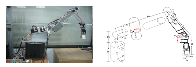
Figure 1 Prototype of robot manipulator with 8DOF.

 Eq. (10) describes the optimization problem to obtain the inverse kinematic solution for minimizing tracking error. To standardize the multi objective optimization problem, the second priority task of the obstacle avoidance in Eq. (11) is modified as follows.

M i n i m i z e Δ q 1 ( k ) , ... , Δ q n ( k )   Φ 2 = 1 min a r o b o t b o b s t a c l e s a ( q ) b 2 MathType@MTEF@5@5@+= feaagKart1ev2aaatCvAUfeBSjuyZL2yd9gzLbvyNv2CaerbuLwBLn hiov2DGi1BTfMBaeXatLxBI9gBaerbd9wDYLwzYbItLDharqqtubsr 4rNCHbGeaGqiVCI8FfYJH8YrFfeuY=Hhbbf9v8qqaqFr0xc9pk0xbb a9q8WqFfeaY=biLkVcLq=JHqpepeea0=as0Fb9pgeaYRXxe9vr0=vr 0=vqpWqaaeaabiGaciaacaqabeaadaqaaqaaaOqaaKqbaoaaxababa GaamytaiaadMgacaWGUbGaamyAaiaad2gacaWGPbGaamOEaiaadwga aeaacqGHuoarcaWGXbWaaSbaaKqbGeaacaaIXaaabeaajuaGdaqada qaaiaadUgaaiaawIcacaGLPaaacaGGSaGaaiOlaiaac6cacaGGUaGa aiilaiabgs5aejaadghadaWgaaqcfasaaiaad6gaaeqaaKqbaoaabm aabaGaam4AaaGaayjkaiaawMcaaaqabaaeaaaaaaaaa8qacaGGGcGa euOPdy0aaSbaaKqbGeaacaaIYaaabeaajuaGcqGH9aqpdaWcaaqaai aaigdaaeaadaWfqaqaaiGac2gacaGGPbGaaiOBaaabaeqabaGaamyy aiabgIGiolaadkhacaWGVbGaamOyaiaad+gacaWG0baabaGaamOyai abgIGiolaad+gacaWGIbGaam4CaiaadshacaWGHbGaam4yaiaadYga caWGLbGaam4Caaaabeaadaqbdaqaaiaadggadaqadaqaaiaadghaai aawIcacaGLPaaacqGHsislcaWGIbaacaGLjWUaayPcSdWaaWbaaeqa juaibaGaaGOmaaaaaaaaaa@7337@ (12)

Solving a multi objective optimization problem is understood as a representative set of Pareto optimal solutions. One of the solving methods is formulating a single objective optimization problem to represent the multi objective optimization by linear scalarization such that optimal solutions to the single-objective optimization problem are Pareto optimal solutions to the multi objective optimization problem. In this study, the multi objective method using linear scalarization for the two task-priorities is described as follows.

M i n i m i z e Δ q 1 ( k ) , ... , Δ q n ( k )   [ w 1 Φ 1 ( r ) + w 2 Φ 2 ( r ) ] MathType@MTEF@5@5@+= feaagKart1ev2aaatCvAUfeBSjuyZL2yd9gzLbvyNv2CaerbuLwBLn hiov2DGi1BTfMBaeXatLxBI9gBaerbd9wDYLwzYbItLDharqqtubsr 4rNCHbGeaGqiVCI8FfYJH8YrFfeuY=Hhbbf9v8qqaqFr0xc9pk0xbb a9q8WqFfeaY=biLkVcLq=JHqpepeea0=as0Fb9pgeaYRXxe9vr0=vr 0=vqpWqaaeaabiGaciaacaqabeaadaqaaqaaaOqaaKqbaoaaxababa GaamytaiaadMgacaWGUbGaamyAaiaad2gacaWGPbGaamOEaiaadwga aeaacqGHuoarcaWGXbWaaSbaaKqbGeaacaaIXaaabeaajuaGdaqada qaaiaadUgaaiaawIcacaGLPaaacaGGSaGaaiOlaiaac6cacaGGUaGa aiilaiabgs5aejaadghadaWgaaqcfasaaiaad6gaaeqaaKqbaoaabm aabaGaam4AaaGaayjkaiaawMcaaaqabaaeaaaaaaaaa8qacaGGGcWa amWaaeaacaWG3bWaaSbaaKqbGeaacaaIXaaabeaajuaGcqqHMoGrda WgaaqcfasaaiaaigdaaeqaaKqbaoaabmaabaGaamOCaaGaayjkaiaa wMcaaiabgUcaRiaadEhadaWgaaqcfasaaiaaikdaaKqbagqaaiabfA 6agnaaBaaajuaibaGaaGOmaaqabaqcfa4aaeWaaeaacaWGYbaacaGL OaGaayzkaaaacaGLBbGaayzxaaaaaa@6301@ (13)

Where the weighting factors of the objectives w i > 0 , i = 1 , 2 MathType@MTEF@5@5@+= feaagKart1ev2aaatCvAUfeBSjuyZL2yd9gzLbvyNv2CaerbuLwBLn hiov2DGi1BTfMBaeXatLxBI9gBaerbd9wDYLwzYbItLDharqqtubsr 4rNCHbGeaGqiVCI8FfYJH8YrFfeuY=Hhbbf9v8qqaqFr0xc9pk0xbb a9q8WqFfeaY=biLkVcLq=JHqpepeea0=as0Fb9pgeaYRXxe9vr0=vr 0=vqpWqaaeaabiGaciaacaqabeaadaqaaqaaaOqaaKqbakaadEhada WgaaqcfasaaiaadMgaaKqbagqaaiabg6da+iaaicdacaGGSaGaamyA aiabg2da9iaaigdacaGGSaGaaGOmaaaa@3FCD@ the parameters of the secularization, and ε-constraint method is applied to this optimization as follows.

M i n i m i z e Δ q 1 ( k ) , ... , Δ q n ( k )   [ w 1 Φ 1 ( r ) + w 2 Φ 2 ( r ) ] MathType@MTEF@5@5@+= feaagKart1ev2aaatCvAUfeBSjuyZL2yd9gzLbvyNv2CaerbuLwBLn hiov2DGi1BTfMBaeXatLxBI9gBaerbd9wDYLwzYbItLDharqqtubsr 4rNCHbGeaGqiVCI8FfYJH8YrFfeuY=Hhbbf9v8qqaqFr0xc9pk0xbb a9q8WqFfeaY=biLkVcLq=JHqpepeea0=as0Fb9pgeaYRXxe9vr0=vr 0=vqpWqaaeaabiGaciaacaqabeaadaqaaqaaaOqaaKqbaoaaxababa GaamytaiaadMgacaWGUbGaamyAaiaad2gacaWGPbGaamOEaiaadwga aeaacqGHuoarcaWGXbWaaSbaaKqbGeaacaaIXaaabeaajuaGdaqada qaaiaadUgaaiaawIcacaGLPaaacaGGSaGaaiOlaiaac6cacaGGUaGa aiilaiabgs5aejaadghadaWgaaqcfasaaiaad6gaaeqaaKqbaoaabm aabaGaam4AaaGaayjkaiaawMcaaaqabaaeaaaaaaaaa8qacaGGGcWa amWaaeaacaWG3bWaaSbaaKqbGeaacaaIXaaabeaajuaGcqqHMoGrda WgaaqcfasaaiaaigdaaeqaaKqbaoaabmaabaGaamOCaaGaayjkaiaa wMcaaiabgUcaRiaadEhadaWgaaqcfasaaiaaikdaaKqbagqaaiabfA 6agnaaBaaajuaibaGaaGOmaaqabaqcfa4aaeWaaeaacaWGYbaacaGL OaGaayzkaaaacaGLBbGaayzxaaaaaa@6301@ (14)

Figure 2 Controller architecture of robot manipulator with 8 DOF.
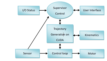
Figure 3 Software architecture of controller.

Subject to r ( t ) X MathType@MTEF@5@5@+= feaagKart1ev2aaatCvAUfeBSjuyZL2yd9gzLbvyNv2CaerbuLwBLn hiov2DGi1BTfMBaeXatLxBI9gBaerbd9wDYLwzYbItLDharqqtubsr 4rNCHbGeaGqiVCI8FfYJH8YrFfeuY=Hhbbf9v8qqaqFr0xc9pk0xbb a9q8WqFfeaY=biLkVcLq=JHqpepeea0=as0Fb9pgeaYRXxe9vr0=vr 0=vqpWqaaeaabiGaciaacaqabeaadaqaaqaaaOqaaKqbakaadkhada qadaqaaiaadshaaiaawIcacaGLPaaacqGHiiIZcaWGybaaaa@3C53@ , Φ i ( r ) ε i MathType@MTEF@5@5@+= feaagKart1ev2aaatCvAUfeBSjuyZL2yd9gzLbvyNv2CaerbuLwBLn hiov2DGi1BTfMBaeXatLxBI9gBaerbd9wDYLwzYbItLDharqqtubsr 4rNCHbGeaGqiVCI8FfYJH8YrFfeuY=Hhbbf9v8qqaqFr0xc9pk0xbb a9q8WqFfeaY=biLkVcLq=JHqpepeea0=as0Fb9pgeaYRXxe9vr0=vr 0=vqpWqaaeaabiGaciaacaqabeaadaqaaqaaaOqaaKqbakabfA6agn aaBaaabaGaamyAaaqabaWaaeWaaeaacaWGYbaacaGLOaGaayzkaaGa eyizImQaeqyTdu2aaSbaaeaacaWGPbaabeaaaaa@3FED@ for i { 1 , 2 } MathType@MTEF@5@5@+= feaagKart1ev2aaatCvAUfeBSjuyZL2yd9gzLbvyNv2CaerbuLwBLn hiov2DGi1BTfMBaeXatLxBI9gBaerbd9wDYLwzYbItLDharqqtubsr 4rNCHbGeaGqiVCI8FfYJH8YrFfeuY=Hhbbf9v8qqaqFr0xc9pk0xbb a9q8WqFfeaY=biLkVcLq=JHqpepeea0=as0Fb9pgeaYRXxe9vr0=vr 0=vqpWqaaeaabiGaciaacaqabeaadaqaaqaaaOqaaKqbakaadMgacq GHiiIZdaGadaqaaiaaigdacaGGSaGaaGOmaaGaay5Eaiaaw2haaaaa @3D43@ where the parameters are the εi upper bounds of the objectives which are Φ i ( r ) MathType@MTEF@5@5@+= feaagKart1ev2aaatCvAUfeBSjuyZL2yd9gzLbvyNv2CaerbuLwBLn hiov2DGi1BTfMBaeXatLxBI9gBaerbd9wDYLwzYbItLDharqqtubsr 4rNCHbGeaGqiVCI8FfYJH8YrFfeuY=Hhbbf9v8qqaqFr0xc9pk0xbb a9q8WqFfeaY=biLkVcLq=JHqpepeea0=as0Fb9pgeaYRXxe9vr0=vr 0=vqpWqaaeaabiGaciaacaqabeaadaqaaqaaaOqaaKqbakabfA6agn aaBaaajuaibaGaamyAaaqabaqcfa4aaeWaaeaacaWGYbaacaGLOaGa ayzkaaaaaa@3C3E@ to be minimized. Is the permissible zone for trajectory tracking tasks. X In this study, a multi objective genetic algorithm (MOGA) method is studied to solve this problem. First, the positioning error is defined as follows.

e ( k ) = ( e x ( k ) ) 2 + ( e y ( k ) ) 2 + ( e z ( k ) ) 2 MathType@MTEF@5@5@+= feaagKart1ev2aaatCvAUfeBSjuyZL2yd9gzLbvyNv2CaerbuLwBLn hiov2DGi1BTfMBaeXatLxBI9gBaerbd9wDYLwzYbItLDharqqtubsr 4rNCHbGeaGqiVCI8FfYJH8YrFfeuY=Hhbbf9v8qqaqFr0xc9pk0xbb a9q8WqFfeaY=biLkVcLq=JHqpepeea0=as0Fb9pgeaYRXxe9vr0=vr 0=vqpWqaaeaabiGaciaacaqabeaadaqaaqaaaOqaaKqbakaadwgada qadaqaaiaadUgaaiaawIcacaGLPaaacqGH9aqpdaGcaaqaamaabmaa baGaamyzamaaBaaajuaibaGaamiEaaqabaqcfa4aaeWaaeaacaWGRb aacaGLOaGaayzkaaaacaGLOaGaayzkaaWaaWbaaKqbGeqabaGaaGOm aaaajuaGcqGHRaWkdaqadaqaaiaadwgadaWgaaqcfasaaiaadMhaae qaaKqbaoaabmaabaGaam4AaaGaayjkaiaawMcaaaGaayjkaiaawMca amaaCaaajuaibeqaaiaaikdaaaqcfaOaey4kaSYaaeWaaeaacaWGLb WaaSbaaKqbGeaacaWG6baabeaajuaGdaqadaqaaiaadUgaaiaawIca caGLPaaaaiaawIcacaGLPaaadaahaaqcfasabeaacaaIYaaaaaqcfa yabaaaaa@55D9@ (15)

Where r r e f ( k ) = [ x r ( k ) y r ( k ) z r ( k ) ] T MathType@MTEF@5@5@+= feaagKart1ev2aaatCvAUfeBSjuyZL2yd9gzLbvyNv2CaerbuLwBLn hiov2DGi1BTfMBaeXatLxBI9gBaerbd9wDYLwzYbItLDharqqtubsr 4rNCHbGeaGqiVCI8FfYJH8YrFfeuY=Hhbbf9v8qqaqFr0xc9pk0xbb a9q8WqFfeaY=biLkVcLq=JHqpepeea0=as0Fb9pgeaYRXxe9vr0=vr 0=vqpWqaaeaabiGaciaacaqabeaadaqaaqaaaOqaaKqbakaadkhada WgaaqcfasaaiaadkhacaWGLbGaamOzaaqabaqcfa4aaeWaaeaacaWG RbaacaGLOaGaayzkaaGaeyypa0deaaaaaaaaa8qadaWadaqaauaabe qabmaaaeaacaWG4bWaaSbaaKqbGeaacaWGYbaabeaajuaGdaqadaqa aiaadUgaaiaawIcacaGLPaaaaeaacaWG5bWaaSbaaKqbGeaacaWGYb aabeaajuaGdaqadaqaaiaadUgaaiaawIcacaGLPaaaaeaacaWG6bWa aSbaaKqbGeaacaWGYbaajuaGbeaadaqadaqaaiaadUgaaiaawIcaca GLPaaaaaaacaGLBbGaayzxaaWaaWbaaeqajuaibaGaamivaaaaaaa@51C3@ the trajectory references and the actual end-effectors’ position are r ( k )   = f ( q ( k ) )   =   [ x ( k ) y ( k ) z ( k ) ] T MathType@MTEF@5@5@+= feaagKart1ev2aaatCvAUfeBSjuyZL2yd9gzLbvyNv2CaerbuLwBLn hiov2DGi1BTfMBaeXatLxBI9gBaerbd9wDYLwzYbItLDharqqtubsr 4rNCHbGeaGqiVCI8FfYJH8YrFfeuY=Hhbbf9v8qqaqFr0xc9pk0xbb a9q8WqFfeaY=biLkVcLq=JHqpepeea0=as0Fb9pgeaYRXxe9vr0=vr 0=vqpWqaaeaabiGaciaacaqabeaadaqaaqaaaOqaaKqbakaadkhada qadaqaaiaadUgaaiaawIcacaGLPaaaqaaaaaaaaaWdbiaacckapaGa eyypa0JaamOzamaabmaabaGaamyCamaabmaabaGaam4AaaGaayjkai aawMcaaaGaayjkaiaawMcaa8qacaGGGcWdaiabg2da98qacaGGGcWa amWaaeaafaqabeqadaaabaGaamiEamaabmaabaGaam4AaaGaayjkai aawMcaaaqaaiaadMhadaqadaqaaiaadUgaaiaawIcacaGLPaaaaeaa caWG6bWaaeWaaeaacaWGRbaacaGLOaGaayzkaaaaaaGaay5waiaaw2 faamaaCaaabeqcfasaaiaadsfaaaaaaa@5331@ Therefore, the tracking for each direction can be defined as e x ( k ) = x r ( k ) x ( k ) , e y ( k ) = y r ( k ) y ( k ) MathType@MTEF@5@5@+= feaagKart1ev2aaatCvAUfeBSjuyZL2yd9gzLbvyNv2CaerbuLwBLn hiov2DGi1BTfMBaeXatLxBI9gBaerbd9wDYLwzYbItLDharqqtubsr 4rNCHbGeaGqiVCI8FfYJH8YrFfeuY=Hhbbf9v8qqaqFr0xc9pk0xbb a9q8WqFfeaY=biLkVcLq=JHqpepeea0=as0Fb9pgeaYRXxe9vr0=vr 0=vqpWqaaeaabiGaciaacaqabeaadaqaaqaaaOqaaKqbacbaaaaaaa aapeGaamyzamaaBaaajuaibaGaamiEaaqcfayabaWaaeWaaeaacaWG RbaacaGLOaGaayzkaaGaeyypa0JaamiEamaaBaaajuaibaGaamOCaa qcfayabaWaaeWaaeaacaWGRbaacaGLOaGaayzkaaGaeyOeI0IaamiE amaabmaabaGaam4AaaGaayjkaiaawMcaaiaacYcacaWGLbWaaSbaaK qbGeaacaWG5baajuaGbeaadaqadaqaaiaadUgaaiaawIcacaGLPaaa cqGH9aqpcaWG5bWaaSbaaKqbGeaacaWGYbaajuaGbeaadaqadaqaai aadUgaaiaawIcacaGLPaaacqGHsislcaWG5bWaaeWaaeaacaWGRbaa caGLOaGaayzkaaaaaa@572C@ and e z ( k ) = z r ( k ) z ( k ) MathType@MTEF@5@5@+= feaagKart1ev2aaatCvAUfeBSjuyZL2yd9gzLbvyNv2CaerbuLwBLn hiov2DGi1BTfMBaeXatLxBI9gBaerbd9wDYLwzYbItLDharqqtubsr 4rNCHbGeaGqiVCI8FfYJH8YrFfeuY=Hhbbf9v8qqaqFr0xc9pk0xbb a9q8WqFfeaY=biLkVcLq=JHqpepeea0=as0Fb9pgeaYRXxe9vr0=vr 0=vqpWqaaeaabiGaciaacaqabeaadaqaaqaaaOqaaKqbacbaaaaaaa aapeGaamyzamaaBaaajuaibaGaamOEaaqcfayabaWaaeWaaeaacaWG RbaacaGLOaGaayzkaaGaeyypa0JaamOEamaaBaaajuaibaGaamOCaa qabaqcfa4aaeWaaeaacaWGRbaacaGLOaGaayzkaaGaeyOeI0IaamOE amaabmaabaGaam4AaaGaayjkaiaawMcaaaaa@468F@ . If the tracking error | e ( k ) | MathType@MTEF@5@5@+= feaagKart1ev2aaatCvAUfeBSjuyZL2yd9gzLbvyNv2CaerbuLwBLn hiov2DGi1BTfMBaeXatLxBI9gBaerbd9wDYLwzYbItLDharqqtubsr 4rNCHbGeaGqiVCI8FfYJH8YrFfeuY=Hhbbf9v8qqaqFr0xc9pk0xbb a9q8WqFfeaY=biLkVcLq=JHqpepeea0=as0Fb9pgeaYRXxe9vr0=vr 0=vqpWqaaeaabiGaciaacaqabeaadaqaaqaaaOqaaKqbacbaaaaaaa aapeWaaqWaaeaacaWGLbWaaeWaaeaacaWGRbaacaGLOaGaayzkaaaa caGLhWUaayjcSdaaaa@3D1E@ is smaller than the permissible value ρ MathType@MTEF@5@5@+= feaagKart1ev2aaatCvAUfeBSjuyZL2yd9gzLbvyNv2CaerbuLwBLn hiov2DGi1BTfMBaeXatLxBI9gBaerbd9wDYLwzYbItLDharqqtubsr 4rNCHbGeaGqiVCI8FfYJH8YrFfeuY=Hhbbf9v8qqaqFr0xc9pk0xbb a9q8WqFfeaY=biLkVcLq=JHqpepeea0=as0Fb9pgeaYRXxe9vr0=vr 0=vqpWqaaeaabiGaciaacaqabeaadaqaaqaaaOqaaKqbacbaaaaaaa aapeGaeqyWdihaaa@3859@ then the end-effectors’ position r ( k ) MathType@MTEF@5@5@+= feaagKart1ev2aaatCvAUfeBSjuyZL2yd9gzLbvyNv2CaerbuLwBLn hiov2DGi1BTfMBaeXatLxBI9gBaerbd9wDYLwzYbItLDharqqtubsr 4rNCHbGeaGqiVCI8FfYJH8YrFfeuY=Hhbbf9v8qqaqFr0xc9pk0xbb a9q8WqFfeaY=biLkVcLq=JHqpepeea0=as0Fb9pgeaYRXxe9vr0=vr 0=vqpWqaaeaabiGaciaacaqabeaadaqaaqaaaOqaaKqbacbaaaaaaa aapeGaamOCamaabmaabaGaam4AaaGaayjkaiaawMcaaaaa@3A09@ is located in the permissible zone ( r ( t ) X ) MathType@MTEF@5@5@+= feaagKart1ev2aaatCvAUfeBSjuyZL2yd9gzLbvyNv2CaerbuLwBLn hiov2DGi1BTfMBaeXatLxBI9gBaerbd9wDYLwzYbItLDharqqtubsr 4rNCHbGeaGqiVCI8FfYJH8YrFfeuY=Hhbbf9v8qqaqFr0xc9pk0xbb a9q8WqFfeaY=biLkVcLq=JHqpepeea0=as0Fb9pgeaYRXxe9vr0=vr 0=vqpWqaaeaabiGaciaacaqabeaadaqaaqaaaOqaaKqbacbaaaaaaa aapeWaaeWaaeaacaWGYbWaaeWaaeaacaWG0baacaGLOaGaayzkaaGa eyicI4SaamiwaaGaayjkaiaawMcaaaaa@3DFC@ .

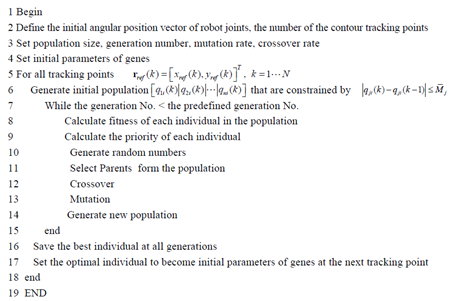
An evolution algorithm (EA) based motion planning method is proposed to produce the motion planning and trajectory tracking with obstacle avoidance. The processes for the proposed EA-based motion planning (EAMP) are described as follows.

  1. An initial population of EA is randomly composed of a large set of gene with chromosomes as described in Figure 4, where k is the time indexing, j is the joint indexing and i represents the index of the gene. The initial population is produced using the stochastic selection. The algorithm allocates a population of gene Pi (0) using the stochastic selection from the permissible set at each step, where Pi (0) is the ith gene, whose chromosomes are [ q 1 i ( 0 ) | q 2 i ( 0 ) | ... | q n i ( 0 ) ] MathType@MTEF@5@5@+= feaagKart1ev2aaatCvAUfeBSjuyZL2yd9gzLbvyNv2CaerbuLwBLn hiov2DGi1BTfMBaeXatLxBI9gBaerbd9wDYLwzYbItLDharqqtubsr 4rNCHbGeaGqiVCI8FfYJH8YrFfeuY=Hhbbf9v8qqaqFr0xc9pk0xbb a9q8WqFfeaY=biLkVcLq=JHqpepeea0=as0Fb9pgeaYRXxe9vr0=vr 0=vqpWqaaeaabiGaciaacaqabeaadaqaaqaaaOqaaKqbaoaadmaaba WaaqGaaeaacaWGXbWaaSbaaKqbGeaacaaIXaGaamyAaaqabaqcfa4a aeWaaeaacaaIWaaacaGLOaGaayzkaaaacaGLiWoadaabcaqaaiaadg hadaWgaaqcfasaaiaaikdacaWGPbaabeaajuaGdaqadaqaaiaaicda aiaawIcacaGLPaaaaiaawIa7aiaac6cacaGGUaGaaiOlamaaeeaaba GaamyCamaaBaaajuaibaGaamOBaiaadMgaaKqbagqaamaabmaabaGa aGimaaGaayjkaiaawMcaaaGaay5bSdaacaGLBbGaayzxaaaaaa@50B7@ which is defined as the gene p i ( 0 ) MathType@MTEF@5@5@+= feaagKart1ev2aaatCvAUfeBSjuyZL2yd9gzLbvyNv2CaerbuLwBLn hiov2DGi1BTfMBaeXatLxBI9gBaerbd9wDYLwzYbItLDharqqtubsr 4rNCHbGeaGqiVCI8FfYJH8YrFfeuY=Hhbbf9v8qqaqFr0xc9pk0xbb a9q8WqFfeaY=biLkVcLq=JHqpepeea0=as0Fb9pgeaYRXxe9vr0=vr 0=vqpWqaaeaabiGaciaacaqabeaadaqaaqaaaOqaaKqbakaadchada WgaaqcfasaaiaadMgaaKqbagqaamaabmaabaGaaGimaaGaayjkaiaa wMcaaaaa@3B7C@ . The gene p i ( 0 ) MathType@MTEF@5@5@+= feaagKart1ev2aaatCvAUfeBSjuyZL2yd9gzLbvyNv2CaerbuLwBLn hiov2DGi1BTfMBaeXatLxBI9gBaerbd9wDYLwzYbItLDharqqtubsr 4rNCHbGeaGqiVCI8FfYJH8YrFfeuY=Hhbbf9v8qqaqFr0xc9pk0xbb a9q8WqFfeaY=biLkVcLq=JHqpepeea0=as0Fb9pgeaYRXxe9vr0=vr 0=vqpWqaaeaabiGaciaacaqabeaadaqaaqaaaOqaaKqbakaadchada WgaaqcfasaaiaadMgaaKqbagqaamaabmaabaGaaGimaaGaayjkaiaa wMcaaaaa@3B7C@ whose chromosomes are constrained in the permissible sets | Δ q j i ( 0 ) |   M ¯ j MathType@MTEF@5@5@+= feaagKart1ev2aaatCvAUfeBSjuyZL2yd9gzLbvyNv2CaerbuLwBLn hiov2DGi1BTfMBaeXatLxBI9gBaerbd9wDYLwzYbItLDharqqtubsr 4rNCHbGeaGqiVCI8FfYJH8YrFfeuY=Hhbbf9v8qqaqFr0xc9pk0xbb a9q8WqFfeaY=biLkVcLq=JHqpepeea0=as0Fb9pgeaYRXxe9vr0=vr 0=vqpWqaaeaabiGaciaacaqabeaadaqaaqaaaOqaaKqbaoaaemaaba GaeyiLdqKaamyCamaaBaaajuaibaGaamOAaiaadMgaaKqbagqaamaa bmaabaGaaGimaaGaayjkaiaawMcaaaGaay5bSlaawIa7aabaaaaaaa aapeGaaiiOa8aacqGHKjYOceWGnbGbaebadaWgaaqcfasaaiaadQga aKqbagqaaaaa@46B3@ .
  2. Filter the gene P i ( k ) = [ q 1 i ( k ) | q 2 i ( k ) | ... | q n i ( k ) ] MathType@MTEF@5@5@+= feaagKart1ev2aaatCvAUfeBSjuyZL2yd9gzLbvyNv2CaerbuLwBLn hiov2DGi1BTfMBaeXatLxBI9gBaerbd9wDYLwzYbItLDharqqtubsr 4rNCHbGeaGqiVCI8FfYJH8YrFfeuY=Hhbbf9v8qqaqFr0xc9pk0xbb a9q8WqFfeaY=biLkVcLq=JHqpepeea0=as0Fb9pgeaYRXxe9vr0=vr 0=vqpWqaaeaabiGaciaacaqabeaadaqaaqaaaOqaaKqbakaadcfada WgaaqcfasaaiaadMgaaKqbagqaamaabmaabaGaam4AaaGaayjkaiaa wMcaaiabg2da9maadmaabaWaaqGaaeaacaWGXbWaaSbaaKqbGeaaca aIXaGaamyAaaqabaqcfa4aaeWaaeaacaWGRbaacaGLOaGaayzkaaaa caGLiWoadaabcaqaaiaadghadaWgaaqcfasaaiaaikdacaWGPbaabe aajuaGdaqadaqaaiaadUgaaiaawIcacaGLPaaaaiaawIa7aiaac6ca caGGUaGaaiOlamaaeeaabaGaamyCamaaBaaajuaibaGaamOBaiaadM gaaKqbagqaamaabmaabaGaam4AaaGaayjkaiaawMcaaaGaay5bSdaa caGLBbGaayzxaaaaaa@5778@ in this population to satisfy the following condition.

Φ 0 ( r ( k ) ) = ( e x ( k ) ) 2 + ( e y ( k ) ) 2 + ( e z ( k ) ) 2         ρ MathType@MTEF@5@5@+= feaagKart1ev2aaatCvAUfeBSjuyZL2yd9gzLbvyNv2CaerbuLwBLn hiov2DGi1BTfMBaeXatLxBI9gBaerbd9wDYLwzYbItLDharqqtubsr 4rNCHbGeaGqiVCI8FfYJH8YrFfeuY=Hhbbf9v8qqaqFr0xc9pk0xbb a9q8WqFfeaY=biLkVcLq=JHqpepeea0=as0Fb9pgeaYRXxe9vr0=vr 0=vqpWqaaeaabiGaciaacaqabeaadaqaaqaaaOqaaKqbakabfA6agn aaBaaajuaibaGaaGimaaqabaqcfa4aaeWaaeaacaWGYbWaaeWaaeaa caWGRbaacaGLOaGaayzkaaaacaGLOaGaayzkaaGaeyypa0ZaaOaaae aadaqadaqaaiaadwgadaWgaaqcfasaaiaadIhaaKqbagqaamaabmaa baGaam4AaaGaayjkaiaawMcaaaGaayjkaiaawMcaamaaCaaajuaibe qaaiaaikdaaaqcfaOaey4kaSYaaeWaaeaacaWGLbWaaSbaaKqbGeaa caWG5baajuaGbeaadaqadaqaaiaadUgaaiaawIcacaGLPaaaaiaawI cacaGLPaaadaahaaqcfasabeaacaaIYaaaaKqbakabgUcaRmaabmaa baGaamyzamaaBaaajuaibaGaamOEaaqcfayabaWaaeWaaeaacaWGRb aacaGLOaGaayzkaaaacaGLOaGaayzkaaWaaWbaaKqbGeqabaGaaGOm aaaaaKqbagqaaabaaaaaaaaapeGaaiiOaiaacckacqGHKjYOcaGGGc GaaiiOaiabeg8aYbaa@62A5@ (16)

Subject to r ( k ) = f ( P i ( k ) ) = f ( [ q 1 i ( k ) | q 2 i ( k ) | ... | q n i ( k ) ] ) MathType@MTEF@5@5@+= feaagKart1ev2aaatCvAUfeBSjuyZL2yd9gzLbvyNv2CaerbuLwBLn hiov2DGi1BTfMBaeXatLxBI9gBaerbd9wDYLwzYbItLDharqqtubsr 4rNCHbGeaGqiVCI8FfYJH8YrFfeuY=Hhbbf9v8qqaqFr0xc9pk0xbb a9q8WqFfeaY=biLkVcLq=JHqpepeea0=as0Fb9pgeaYRXxe9vr0=vr 0=vqpWqaaeaabiGaciaacaqabeaadaqaaqaaaOqaaKqbakaadkhada qadaqaaiaadUgaaiaawIcacaGLPaaacqGH9aqpcaWGMbWaaeWaaeaa caWGqbWaaSbaaKqbGeaacaWGPbaabeaajuaGdaqadaqaaiaadUgaai aawIcacaGLPaaaaiaawIcacaGLPaaacqGH9aqpcaWGMbWaaeWaaeaa daWadaqaamaaeiaabaGaamyCamaaBaaajuaibaGaaGymaiaadMgaae qaaKqbaoaabmaabaGaam4AaaGaayjkaiaawMcaaaGaayjcSdWaaqGa aeaacaWGXbWaaSbaaKqbGeaacaaIYaGaamyAaaqabaqcfa4aaeWaae aacaWGRbaacaGLOaGaayzkaaaacaGLiWoacaGGUaGaaiOlaiaac6ca daabbaqaaiaadghadaWgaaqcfasaaiaad6gacaWGPbaabeaajuaGda qadaqaaiaadUgaaiaawIcacaGLPaaaaiaawEa7aaGaay5waiaaw2fa aaGaayjkaiaawMcaaaaa@60D6@ | q j i ( k ) q i ( k 1 ) | M ¯ j ,     j =   1... n ,     i = 1... N MathType@MTEF@5@5@+= feaagKart1ev2aaatCvAUfeBSjuyZL2yd9gzLbvyNv2CaerbuLwBLn hiov2DGi1BTfMBaeXatLxBI9gBaerbd9wDYLwzYbItLDharqqtubsr 4rNCHbGeaGqiVCI8FfYJH8YrFfeuY=Hhbbf9v8qqaqFr0xc9pk0xbb a9q8WqFfeaY=biLkVcLq=JHqpepeea0=as0Fb9pgeaYRXxe9vr0=vr 0=vqpWqaaeaabiGaciaacaqabeaadaqaaqaaaOqaaKqbaoaaemaaba GaamyCamaaBaaajuaibaGaamOAaiaadMgaaeqaaKqbaoaabmaabaGa am4AaaGaayjkaiaawMcaaiabgkHiTiaadghadaWgaaqcfasaaiaadM gaaeqaaKqbaoaabmaabaGaam4AaiabgkHiTiaaigdaaiaawIcacaGL PaaaaiaawEa7caGLiWoacqGHKjYOceWGnbGbaebadaWgaaqaaKqbGi aadQgajuaGcaGGSaaeaaaaaaaaa8qacaGGGcGaaiiOaaWdaeqaaiaa dQgacqGH9aqppeGaaiiOa8aacaaIXaGaaiOlaiaac6cacaGGUaGaam OBaiaacYcapeGaaiiOaiaacckacaWGPbGaeyypa0JaaGymaiaac6ca caGGUaGaaiOlaiaad6eaaaa@5EC1@ where n is the number of joints, N is the number of the population and ρ is the radius of the permissible zone. After this filtering process, the permissible chromosomes should satisfy the condition where the end-effector positions are located in the region of Φ 0 ( r ( k ) ) ρ MathType@MTEF@5@5@+= feaagKart1ev2aaatCvAUfeBSjuyZL2yd9gzLbvyNv2CaerbuLwBLn hiov2DGi1BTfMBaeXatLxBI9gBaerbd9wDYLwzYbItLDharqqtubsr 4rNCHbGeaGqiVCI8FfYJH8YrFfeuY=Hhbbf9v8qqaqFr0xc9pk0xbb a9q8WqFfeaY=biLkVcLq=JHqpepeea0=as0Fb9pgeaYRXxe9vr0=vr 0=vqpWqaaeaabiGaciaacaqabeaadaqaaqaaaOqaaKqbakabfA6agn aaBaaajuaibaGaaGimaaqabaqcfa4aaeWaaeaacaWGYbWaaeWaaeaa caWGRbaacaGLOaGaayzkaaaacaGLOaGaayzkaaGaeyizImQaeqyWdi haaa@41F8@ .

  1. The objective function w 1 Φ 1 ( r ) + w 2 Φ 2 ( r ) MathType@MTEF@5@5@+= feaagKart1ev2aaatCvAUfeBSjuyZL2yd9gzLbvyNv2CaerbuLwBLn hiov2DGi1BTfMBaeXatLxBI9gBaerbd9wDYLwzYbItLDharqqtubsr 4rNCHbGeaGqiVCI8FfYJH8YrFfeuY=Hhbbf9v8qqaqFr0xc9pk0xbb a9q8WqFfeaY=biLkVcLq=JHqpepeea0=as0Fb9pgeaYRXxe9vr0=vr 0=vqpWqaaeaabiGaciaacaqabeaadaqaaqaaaOqaaKqbakaadEhada WgaaqaaKqbGiaaigdajuaGcqqHMoGrdaWgaaqcfasaaiaaigdaaeqa aKqbaoaabmaabaGaamOCaaGaayjkaiaawMcaaaqabaGaey4kaSIaam 4DamaaBaaajuaibaGaaGOmaaqabaqcfaOaeuOPdy0aaSbaaKqbGeaa caaIYaaajuaGbeaadaqadaqaaiaadkhaaiaawIcacaGLPaaaaaa@47A9@ is used to evaluate the fitness of each individual in this population. The set of fitness values are used to sort the population, eliminate the badly-fitted individuals, mate the best-fitted chromosomes, and then propagate the “good” genes (parameter combinations) to the upcoming generation. These processes are repeated until reaching a certain number of generations. The procedures of the RGA are described as follows.
  2. Compute the fitness function: the fitness values are used to sort the population, eliminate the badly-fitted individuals; the individual with the higher fitness function has the better survival chance. In this case, the fitness function is defined as follows

F i t ( P i ( k ) ) = 1 / ( w 1 Φ 1 ( P i ( k ) ) + w 2 Φ 2 ( P i ( k ) ) ) MathType@MTEF@5@5@+= feaagKart1ev2aaatCvAUfeBSjuyZL2yd9gzLbvyNv2CaerbuLwBLn hiov2DGi1BTfMBaeXatLxBI9gBaerbd9wDYLwzYbItLDharqqtubsr 4rNCHbGeaGqiVCI8FfYJH8YrFfeuY=Hhbbf9v8qqaqFr0xc9pk0xbb a9q8WqFfeaY=biLkVcLq=JHqpepeea0=as0Fb9pgeaYRXxe9vr0=vr 0=vqpWqaaeaabiGaciaacaqabeaadaqaaqaaaOqaaKqbakaadAeaca WGPbGaamiDamaabmaabaGaamiuamaaBaaajuaibaGaamyAaaqabaqc fa4aaeWaaeaacaWGRbaacaGLOaGaayzkaaaacaGLOaGaayzkaaGaey ypa0JaaGymaiaac+cadaqadaqaaiaadEhadaWgaaqcfasaaiaaigda aeqaaKqbakabfA6agnaaBaaajuaibaGaaGymaaqabaqcfa4aaeWaae aacaWGqbWaaSbaaKqbGeaacaWGPbaabeaajuaGdaqadaqaaiaadUga aiaawIcacaGLPaaaaiaawIcacaGLPaaacqGHRaWkcaWG3bWaaSbaaK qbGeaacaaIYaaabeaajuaGcqqHMoGrdaWgaaqcfasaaiaaikdaaKqb agqaamaabmaabaGaamiuamaaBaaajuaibaGaamyAaaqabaqcfa4aae WaaeaacaWGRbaacaGLOaGaayzkaaaacaGLOaGaayzkaaaacaGLOaGa ayzkaaaaaa@5D3E@ (17)

  1. Selection: determine pairs of genes for mating. The gene with higher fitness value has the higher priority to become the parents for the evolution.
  2. Crossover with the random selection: the genes after the selection operation can produce the next generation using the crossover operation. Whether the crossover operation performs is determined by the crossover rate and the crossover rate is defined as 0.8 in this study. The crossover method used in this study is a linear combination of two vectors (chromosomes) with two random weighting variables as follows.

C 1 =   α . P 1 + ( 1 α ) . P 2 C 2 =   β . P 1 + ( 1 β ) . P 2 MathType@MTEF@5@5@+= feaagKart1ev2aaatCvAUfeBSjuyZL2yd9gzLbvyNv2CaerbuLwBLn hiov2DGi1BTfMBaeXatLxBI9gBaerbd9wDYLwzYbItLDharqqtubsr 4rNCHbGeaGqiVCI8FfYJH8YrFfeuY=Hhbbf9v8qqaqFr0xc9pk0xbb a9q8WqFfeaY=biLkVcLq=JHqpepeea0=as0Fb9pgeaYRXxe9vr0=vr 0=vqpWqaaeaabiGaciaacaqabeaadaqaaqaaaOabaeqabaqcfaOaam 4qamaaBaaajuaibaGaaGymaaqabaqcfaOaeyypa0deaaaaaaaaa8qa caGGGcGaeqySdeMaaiOlaiaadcfadaWgaaqcfasaaiaaigdaaKqbag qaaiabgUcaRmaabmaabaGaaGymaiabgkHiTiabeg7aHbGaayjkaiaa wMcaaiaac6cacaWGqbWaaSbaaKqbGeaacaaIYaaabeaaaKqbagaaca WGdbWaaSbaaKqbGeaacaaIYaaabeaajuaGcqGH9aqpcaGGGcGaeqOS diMaaiOlaiaadcfadaWgaaqcfasaaiaaigdaaeqaaKqbakabgUcaRm aabmaabaGaaGymaiabgkHiTiabek7aIbGaayjkaiaawMcaaiaac6ca caWGqbWaaSbaaKqbGeaacaaIYaaajuaGbeaaaaaa@5AD9@ (18)

Where P1 and P2 are the gene of the parents; 1 C and 2 C are the gene of the children; , αβ are the uniformly distributed random variables between 0 and 1.

  1. Gaussian mutation operation: if the offspring are determined by the crossover and selection operations, the optimization may fall into local minimum. Using the mutation operation can maintain genetic diversity from one generation of a population to the next. Mutation occurs during evolution according to mutation probability. The mutation probability should be set low to avoid making the RGA turn into a primitive random search and the mutation probability is defined as 0.03 in this work. If the gene is chosen to perform the mutation operation, its chromosomes are obtained as follows.

q j i ( k ) = q j i ( k 1 ) + Y . M ¯ j MathType@MTEF@5@5@+= feaagKart1ev2aaatCvAUfeBSjuyZL2yd9gzLbvyNv2CaerbuLwBLn hiov2DGi1BTfMBaeXatLxBI9gBaerbd9wDYLwzYbItLDharqqtubsr 4rNCHbGeaGqiVCI8FfYJH8YrFfeuY=Hhbbf9v8qqaqFr0xc9pk0xbb a9q8WqFfeaY=biLkVcLq=JHqpepeea0=as0Fb9pgeaYRXxe9vr0=vr 0=vqpWqaaeaabiGaciaacaqabeaadaqaaqaaaOqaaKqbakaadghada WgaaqcfasaaiaadQgacaWGPbaajuaGbeaadaqadaqaaiaadUgaaiaa wIcacaGLPaaacqGH9aqpcaWGXbWaaSbaaKqbGeaacaWGQbGaamyAaa qcfayabaWaaeWaaeaacaWGRbGaeyOeI0IaaGymaaGaayjkaiaawMca aiabgUcaRiaadMfacaGGUaGabmytayaaraWaaSbaaKqbGeaacaWGQb aabeaaaaa@4A13@ (19)

Where Y is a random variable of the Gaussian probability distribution between -1 and 1 M ¯ j MathType@MTEF@5@5@+= feaagKart1ev2aaatCvAUfeBSjuyZL2yd9gzLbvyNv2CaerbuLwBLn hiov2DGi1BTfMBaeXatLxBI9gBaerbd9wDYLwzYbItLDharqqtubsr 4rNCHbGeaGqiVCI8FfYJH8YrFfeuY=Hhbbf9v8qqaqFr0xc9pk0xbb a9q8WqFfeaY=biLkVcLq=JHqpepeea0=as0Fb9pgeaYRXxe9vr0=vr 0=vqpWqaaeaabiGaciaacaqabeaadaqaaqaaaOqaaKqbakqad2eaga qeamaaBaaajuaibaGaamOAaaqabaaaaa@38A1@ is the upper bound of the angular change for the Joint j in one step.

  1. Reproduction with elitist strategy: after the above RGA operations, two elites in the parents’ generation are guaranteed to survive to the next generation.

Figure 4 Illustration of the i-th gene at the k-th sampling.

Ea-based motion planning for redundant robots based on cuda

Genetic algorithm (GA) is a stochastic optimization method for solving many practical problems in engineering, science and business domains, but its execution time may become a limiting factor for some huge optimization problems. Fortunately, the evolution of natural population is very suitable with a parallel architecture, because the most time-consuming fitness evaluations can be performed independently for each individual in population. There are various types of parallelization in GAs: master-slave models, coarse-grained models, fine-grained models, hierarchical models, island models, and hybrid models. The emergence of many-core architectures for GPGPU provides the opportunity to significantly reduce the runtime of many complicated bioinformatics algorithms, such as Sequence and Genome Analysis.31 Using CUDA supplies the system based on commonly available and inexpensive hardware (CPU and GPUs) with more powerful high-performance computing power, which are generally not provided by conventional general-purpose processors. To obtain the optimal inverse kinematic solution for motion planning of a redundant robot with obstacle avoidance, the computation load is very large if the grid search algorithm is used. The motivation of this work is to use a real-coded genetic algorithm (or called evolutionary algorithm, EA) to replace the grid search algorithm to speed up the computation. Genetic algorithm (GA) is a stochastic optimization technique based on the idea of natural evolution and its search process based on natural selection developed by Holland.29 The original GA operates using binary code of chromosomes, but RGA or evolutionary algorithm (EA) uses real-coded chromosomes.30,31 Figure 5 shows the procedure for the EA-based motion-planning method and the optimal solution [ q 1 i ( k + 1 ) | q 2 i ( k 1 ) | ... | q n i ( k + 1 ) ] MathType@MTEF@5@5@+= feaagKart1ev2aaatCvAUfeBSjuyZL2yd9gzLbvyNv2CaerbuLwBLn hiov2DGi1BTfMBaeXatLxBI9gBaerbd9wDYLwzYbItLDharqqtubsr 4rNCHbGeaGqiVCI8FfYJH8YrFfeuY=Hhbbf9v8qqaqFr0xc9pk0xbb a9q8WqFfeaY=biLkVcLq=JHqpepeea0=as0Fb9pgeaYRXxe9vr0=vr 0=vqpWqaaeaabiGaciaacaqabeaadaqaaqaaaOqaaKqbaoaadmaaba WaaqGaaeaacaWGXbWaaSbaaKqbGeaacaaIXaGaamyAaaqcfayabaWa aWbaaeqabaGaeyOiGClaamaabmaabaGaam4AaiabgUcaRiaaigdaai aawIcacaGLPaaaaiaawIa7amaaeiaabaGaamyCamaaBaaajuaibaGa aGOmaiaadMgaaKqbagqaamaaCaaabeqaaiabgkci3caadaqadaqaai aadUgacqGHsislcaaIXaaacaGLOaGaayzkaaaacaGLiWoacaGGUaGa aiOlaiaac6cadaabbaqaaiaadghadaWgaaqcfasaaiaad6gacaWGPb aabeaajuaGdaahaaqabeaacqGHIaYTaaWaaeWaaeaacaWGRbGaey4k aSIaaGymaaGaayjkaiaawMcaaaGaay5bSdaacaGLBbGaayzxaaaaaa@5B30@ are determined at each tracking points in sequence. To implement real-time motion planning with obstacle avoidance, the EAMP is implemented on the CUDA target. Figure 6 shows the flowchart of CUDA for the proposed EAMP. In this study, the code is developed on Lab view IDE, but the CUDA code is performed in the GPU and only supported in C language. Therefore, the CUDA kernel code should be transferred into a DLL file first and then it can be executed in the GPU as the main code (in the host) calls the DLL function file. If the main code is executed in Labview to call the initializing population program (DLL file), then the DLL file would copy data from host memory to the global memory in the GPU, where the program is performed using CUDA kernel. After the CUDA code is finished in the GPU, the program would copy the result from the global memory to the host memory and finish the initial population process. Figure 7 shows the flowchart of the RGAMP in Lab view and the program from left to right are initial population, fitness function calculation, tournament selection, crossover and mutation. The main idea and the detail functions are described as follows.

Initial population using CUDA

The CUDA thread is different from PC thread. In order to generate the initial population in parallelism, the first thing is to determine how many core needed to use. In this study, the number of CUDA thread depends on the number of chromosomes as shown in Figure 8. The main idea is to generate a lot of random value by M cores on CUDA target and each core generates random values using “FOR” loop where N is determined by the DOF of the redundant robot; MN × random values are generated finally. The pseudo random number generator (PRNG) is very important for the proposed Method, because the GPU cannot generate random seeds by time and random seeds are needed to be generated on host. There are many different ways for PRNG.32 Before 2010, CUDA libraries did not include the function for generating random numbers, so the kernel has to generate random numbers using an original process. CUDA SDK comes with a sample random number generator based on Messene twister proposed by Matsumoto et al.34-36 The process is to operate the random seed array in the global memory, and then an array of random numbers, based on the seed array, is produced to the shared memory. In 2010 August, CUDA 3.2 released CURAND, a library for PRNG using Xorwow generator was selected as the PRNG standard of CUDA.36 XORWOW PRNG is introduced by Marsaglia in 2003 to add xor-shift with Weyl sequence.36 First, the PRNG is performed in the host for the proposed method, where the random numbers are produced by CPU. As shown in Figure 8, the random numbers are generated using standard C language routines in the host. This includes the set of random numbers, N r a n d o m , MathType@MTEF@5@5@+= feaagKart1ev2aaatCvAUfeBSjuyZL2yd9gzLbvyNv2CaerbuLwBLn hiov2DGi1BTfMBaeXatLxBI9gBaerbd9wDYLwzYbItLDharqqtubsr 4rNCHbGeaGqiVCI8FfYJH8YrFfeuY=Hhbbf9v8qqaqFr0xc9pk0xbb a9q8WqFfeaY=biLkVcLq=JHqpepeea0=as0Fb9pgeaYRXxe9vr0=vr 0=vqpWqaaeaabiGaciaacaqabeaadaqaaqaaaOqaaKqbakaad6eada WgaaqaaKqbGiaadkhacaWGHbGaamOBaiaadsgacaWGVbGaamyBaKqb akaacYcaaeqaaaaa@3E78@ as follows.

Figure 5 Procedure for the EAMP.

N r a n d o m = N r _ x o v e r , N r _ m u t a t e , N r _ s e l e c t MathType@MTEF@5@5@+= feaagKart1ev2aaatCvAUfeBSjuyZL2yd9gzLbvyNv2CaerbuLwBLn hiov2DGi1BTfMBaeXatLxBI9gBaerbd9wDYLwzYbItLDharqqtubsr 4rNCHbGeaGqiVCI8FfYJH8YrFfeuY=Hhbbf9v8qqaqFr0xc9pk0xbb a9q8WqFfeaY=biLkVcLq=JHqpepeea0=as0Fb9pgeaYRXxe9vr0=vr 0=vqpWqaaeaabiGaciaacaqabeaadaqaaqaaaOqaaKqbakaad6eada WgaaqaaKqbGiaadkhacaWGHbGaamOBaiaadsgacaWGVbGaamyBaaqc fayabaGaeyypa0JaamOtamaaBaaajuaibaGaamOCaiaac+facaWG4b Gaam4BaiaadAhacaWGLbGaamOCaaqcfayabaGaaiilaiaad6eadaWg aaqcfasaaiaadkhacaGGFbGaamyBaiaadwhacaWG0bGaamyyaiaads hacaWGLbaajuaGbeaacaGGSaGaamOtamaaBaaajuaibaGaamOCaiaa c+facaWGZbGaamyzaiaadYgacaWGLbGaam4yaiaadshaaKqbagqaaa aa@5AE5@ Where N r _ x o v e r , N r _ m u t a t e , N r _ s e l e c t MathType@MTEF@5@5@+= feaagKart1ev2aaatCvAUfeBSjuyZL2yd9gzLbvyNv2CaerbuLwBLn hiov2DGi1BTfMBaeXatLxBI9gBaerbd9wDYLwzYbItLDharqqtubsr 4rNCHbGeaGqiVCI8FfYJH8YrFfeuY=Hhbbf9v8qqaqFr0xc9pk0xbb a9q8WqFfeaY=biLkVcLq=JHqpepeea0=as0Fb9pgeaYRXxe9vr0=vr 0=vqpWqaaeaabiGaciaacaqabeaadaqaaqaaaOqaaKqbakaad6eada WgaaqcfasaaiaadkhacaGGFbGaamiEaiaad+gacaWG2bGaamyzaiaa dkhaaKqbagqaaiaacYcacaWGobWaaSbaaKqbGeaacaWGYbGaai4xai aad2gacaWG1bGaamiDaiaadggacaWG0bGaamyzaaqcfayabaGaaiil aiaad6eadaWgaaqcfasaaiaadkhacaGGFbGaam4CaiaadwgacaWGSb GaamyzaiaadogacaWG0baajuaGbeaaaaa@5290@ are the sets of random numbers required by crossover, mutation, and selection stages. For each generation, the random numbers are generated in the host and they are copied to the device for the computation of the proposed method. Each core obtains the random seeds from the seed memory and produces the random numbers using the random seeds. The “for” loop generates N random values and transmits them to the chromosome memory by specific arrangement ( i * N + j ) MathType@MTEF@5@5@+= feaagKart1ev2aaatCvAUfeBSjuyZL2yd9gzLbvyNv2CaerbuLwBLn hiov2DGi1BTfMBaeXatLxBI9gBaerbd9wDYLwzYbItLDharqqtubsr 4rNCHbGeaGqiVCI8FfYJH8YrFfeuY=Hhbbf9v8qqaqFr0xc9pk0xbb a9q8WqFfeaY=biLkVcLq=JHqpepeea0=as0Fb9pgeaYRXxe9vr0=vr 0=vqpWqaaeaabiGaciaacaqabeaadaqaaqaaaOqaaKqbaoaabmaaba GaamyAaiaacQcacaGGobGaey4kaSIaaiOAaaGaayjkaiaawMcaaaaa @3C40@ . The index i is the number of the current core, the index j is the number of the joint.

Calculate fitness function using CUDA Using CUDA

The GPU with many cores could calculate the fitness values for each chromosome in parallelism. Figure 9 shows that the core number is determined by Number of chromosome. For each core, the first thing is to calculate fitness value of each chromosome from the memory space and the next step is to calculate the position of end-effort of robot manipulator. Then, the fitness values are transmitted to the GPU memory and the GPU returns M fitness values for each chromosome.

Selection and crossover for the selection operation

The tournament selection is used to choose the better chromosomes and put them into the crossover pool. The single-point crossover method is used for the EA. The main idea of CUDA code is shown in Figure 10, where each core exchanges its genes from two chromosomes. Thus, this component only employs M/2 cores and each core obtains the joint parameters using the selection and crossover operations from the memories of chromosome1 and chromosome 2, respectively. The crossover rate is designed as 0.8 in this study. First, the program produces a random value and compares it with the crossover rate, where the random value is used to determinate whether the crossover process is performed or not. Second, if the crossover rate is bigger than the random number, then the crossover process is achieved. If the crossover condition is satisfied, the program produces a random crossover point. Then, the “for” loop function is used to perform the crossover operation, where the elements of chromosome 1 and chromosome 2 are exchanged before the index of the crossover point and they are remained as the same after the index of the crossover point. Finally, the GPU transfers the data back to new Chromosome1 memory and the Host obtains M chromosomes.

Figure 6 Flowchart of genetic algorithms based on CUDA.

Mutation for the mutation operation

The component generates N random value for each thread and makes each gene have an opportunity to mutation. Figure 11 shows the main idea and the mutation rate is configured 0.03 in this study. First, a random value is generated by the program. Second, if the mutation rate is bigger than the random number, then the mutation process is achieved. As the mutation condition is satisfied, the GPU regenerates a new gene using | Δ q j i ( 0 ) | M ¯ j MathType@MTEF@5@5@+= feaagKart1ev2aaatCvAUfeBSjuyZL2yd9gzLbvyNv2CaerbuLwBLn hiov2DGi1BTfMBaeXatLxBI9gBaerbd9wDYLwzYbItLDharqqtubsr 4rNCHbGeaGqiVCI8FfYJH8YrFfeuY=Hhbbf9v8qqaqFr0xc9pk0xbb a9q8WqFfeaY=biLkVcLq=JHqpepeea0=as0Fb9pgeaYRXxe9vr0=vr 0=vqpWqaaeaabiGaciaacaqabeaadaqaaqaaaOqaaKqbaoaaemaaba GaeyiLdqKaamyCamaaBaaajuaibaGaamOAaiaadMgaaKqbagqaamaa bmaabaGaaGimaaGaayjkaiaawMcaaaGaay5bSlaawIa7aiabgsMiJk qad2eagaqeamaaBaaajuaibaGaamOAaaqcfayabaaaaa@4560@ randomly and transmits the chromosome data into the chromosome memory. For each generation of the EAMP, the crossover, mutation, and selection operations are performed in parallel for the device. The parallel computing processes in the device are described as follows.

  1. Launch GPU Kernel to calculate the fitness of each individual in parallel and copy the fitness values from the GPU to the HOST for comparison.
  2. Reproduction copies the random angular solution in the permissible range from the random pool to the device.
  3. Launch GPU Kernel and generate the random numbers in parallel for the crossover and mutation operations.
  4. Launch GPU Kernel to perform the crossover operation for the EAMP in parallel.
  5. Launch GPU Kernel to perform the mutation operation for the EAMP in parallel.
  6. Initialize the offspring in the next generation and return to Step 1. Finally, the host is used to receive the optimal result where the individual with the best fitness from the device.

Experimental result and discussions

To check the feasibility of real-time motion planning, a trajectory planning task with obstacle avoidance is designed to discuss the positioning accuracy and computation performance for the proposed method.

System description in this study

A robot manipulator with 8 DOFs is designed as shown in Figure 1. Tables 1 & 2 show the specification of the motors used for the system and the D-H parameters of the 8-DOF robot manipulator. Figure 2 shows the control architecture of this robot manipulator, where an NI Compact RIO 9074 is used as the real-time embedded controller for the whole system. The Compact RIO (cRIO) is a combination of a real-time controller, reconfigurable IO Modules (RIO), FPGA module and an Ethernet expansion chassis. The modules NI 9512, 9516 and 9505 are installed in the cRIO 9074 for the purposes of controlling servo motors and DC motors in P-command, I-command drive and PWM-command. The motion commands, which are computed in the PC, are transmitted to cRIO via the internet. In this study, a real-time control code is developed in Lab VIEW and embedded in cRIO 9074 for the real-time implementation. The control architecture is divided into three parts, which are the supervisor control, the trajectory generator, and the hardware-in-loop (HIL) control, and Figure 3 shows the block diagram of the whole system. The user can set the parameters into the system by the supervisor control block, such as the departure and destination, the increment or velocity constraints. After that, the supervisor control block transfers the command to the trajectory generator to produce the trajectory planning path. Finally, the HIL code in cRIO 9074 is used to make the robot manipulator track the desired trajectory and perform the priority task such as obstacle avoidance. 4.2 Motion planning using CUDA architecture the proposed EAMP method is studied to solve this problem to implement Realtime motion planning. The fitness function of the RGA motion planning with avoidance obstacle method is shown in Eq. (14). Table 3 describes the robot parameters for this experimental case study. The initial position of the end-effector is r ( 0 ) = [ 17.0 , 57.6.30.5 ] T MathType@MTEF@5@5@+= feaagKart1ev2aaatCvAUfeBSjuyZL2yd9gzLbvyNv2CaerbuLwBLn hiov2DGi1BTfMBaeXatLxBI9gBaerbd9wDYLwzYbItLDharqqtubsr 4rNCHbGeaGqiVCI8FfYJH8YrFfeuY=Hhbbf9v8qqaqFr0xc9pk0xbb a9q8WqFfeaY=biLkVcLq=JHqpepeea0=as0Fb9pgeaYRXxe9vr0=vr 0=vqpWqaaeaabiGaciaacaqabeaadaqaaqaaaOqaaKqbakaadkhada qadaqaaiaaicdaaiaawIcacaGLPaaacqGH9aqpdaWadaqaaiaaigda caaI3aGaaiOlaiaaicdacaGGSaGaaGynaiaaiEdacaGGUaGaaGOnai aac6cacaaIZaGaaGimaiaac6cacaaI1aaacaGLBbGaayzxaaWaaWba aeqajuaibaGaamivaaaaaaa@47F8@ (mm) with q ( 0 ) = [ 0 0 90 0 50 0 0 0 50 0 0 0 25 0 0 0 ] T MathType@MTEF@5@5@+= feaagKart1ev2aaatCvAUfeBSjuyZL2yd9gzLbvyNv2CaerbuLwBLn hiov2DGi1BTfMBaeXatLxBI9gBaerbd9wDYLwzYbItLDharqqtubsr 4rNCHbGeaGqiVCI8FfYJH8YrFfeuY=Hhbbf9v8qqaqFr0xc9pk0xbb a9q8WqFfeaY=biLkVcLq=JHqpepeea0=as0Fb9pgeaYRXxe9vr0=vr 0=vqpWqaaeaabiGaciaacaqabeaadaqaaqaaaOqaaKqbakaadghada qadaqaaiaaicdaaiaawIcacaGLPaaacqGH9aqpdaWadaqaauaabeqa bGaaaaaabaGaaGimamaaCaaabeqcfasaaiaaicdaaaaajuaGbaGaey OeI0IaaGyoaiaaicdadaahaaqabKqbGeaacaaIWaaaaaqcfayaaiab gkHiTiaaiwdacaaIWaWaaWbaaKqbGeqabaGaaGimaaaaaKqbagaaca aIWaWaaWbaaKqbGeqabaGaaGimaaaaaKqbagaacqGHsislcaaI1aGa aGimamaaCaaajuaibeqaaiaaicdaaaaajuaGbaGaaGimamaaCaaaju aibeqaaiaaicdaaaaajuaGbaGaeyOeI0IaaGOmaiaaiwdadaahaaqc fasabeaacaaIWaaaaaqcfayaaiaaicdadaahaaqabKqbGeaacaaIWa aaaaaaaKqbakaawUfacaGLDbaadaahaaqcfasabeaacaWGubaaaaaa @5732@ the first step is to make the end-effector follow a straight-line trajectory between [ 17.0 , 57.6 , 30.5 ] MathType@MTEF@5@5@+= feaagKart1ev2aaatCvAUfeBSjuyZL2yd9gzLbvyNv2CaerbuLwBLn hiov2DGi1BTfMBaeXatLxBI9gBaerbd9wDYLwzYbItLDharqqtubsr 4rNCHbGeaGqiVCI8FfYJH8YrFfeuY=Hhbbf9v8qqaqFr0xc9pk0xbb a9q8WqFfeaY=biLkVcLq=JHqpepeea0=as0Fb9pgeaYRXxe9vr0=vr 0=vqpWqaaeaabiGaciaacaqabeaadaqaaqaaaOqaaKqbaoaadmaaba GaaGymaiaaiEdacaGGUaGaaGimaiaacYcacaaI1aGaaG4naiaac6ca caaI2aGaaiilaiaaiodacaaIWaGaaiOlaiaaiwdaaiaawUfacaGLDb aaaaa@428D@ and [ 11 , 110 , 40 ] MathType@MTEF@5@5@+= feaagKart1ev2aaatCvAUfeBSjuyZL2yd9gzLbvyNv2CaerbuLwBLn hiov2DGi1BTfMBaeXatLxBI9gBaerbd9wDYLwzYbItLDharqqtubsr 4rNCHbGeaGqiVCI8FfYJH8YrFfeuY=Hhbbf9v8qqaqFr0xc9pk0xbb a9q8WqFfeaY=biLkVcLq=JHqpepeea0=as0Fb9pgeaYRXxe9vr0=vr 0=vqpWqaaeaabiGaciaacaqabeaadaqaaqaaaOqaaKqbaoaadmaaba GaaGymaiaaigdacaGGSaGaaGymaiaaigdacaaIWaGaaiilaiaaisda caaIWaaacaGLBbGaayzxaaaaaa@3EE9@ . Therefore, the reference tracking point in Cartesian space can be obtained by

r r e f ( k ) = r 0 + r d r 0 N × k ,       k = 1... N MathType@MTEF@5@5@+= feaagKart1ev2aaatCvAUfeBSjuyZL2yd9gzLbvyNv2CaerbuLwBLn hiov2DGi1BTfMBaeXatLxBI9gBaerbd9wDYLwzYbItLDharqqtubsr 4rNCHbGeaGqiVCI8FfYJH8YrFfeuY=Hhbbf9v8qqaqFr0xc9pk0xbb a9q8WqFfeaY=biLkVcLq=JHqpepeea0=as0Fb9pgeaYRXxe9vr0=vr 0=vqpWqaaeaabiGaciaacaqabeaadaqaaqaaaOqaaKqbakaadkhada WgaaqcfasaaiaadkhacaWGLbGaamOzaaqabaqcfa4aaeWaaeaacaWG RbaacaGLOaGaayzkaaGaeyypa0JaamOCamaaBaaajuaibaGaaGimaa qcfayabaGaey4kaSYaaSaaaeaacaWGYbWaaSbaaKqbGeaacaWGKbaa beaajuaGcqGHsislcaWGYbWaaSbaaKqbGeaacaaIWaaabeaaaKqbag aacaWGobaaaiabgEna0kaadUgacaGGSaaeaaaaaaaaa8qacaGGGcGa aiiOaiaacckapaGaam4Aaiabg2da9iaaigdacaGGUaGaaiOlaiaac6 cacaWGobaaaa@560F@ (21)

where r 0 = [ 17 57.6 30.5 ] T , r d = [ 11 110 40 ] T MathType@MTEF@5@5@+= feaagKart1ev2aaatCvAUfeBSjuyZL2yd9gzLbvyNv2CaerbuLwBLn hiov2DGi1BTfMBaeXatLxBI9gBaerbd9wDYLwzYbItLDharqqtubsr 4rNCHbGeaGqiVCI8FfYJH8YrFfeuY=Hhbbf9v8qqaqFr0xc9pk0xbb a9q8WqFfeaY=biLkVcLq=JHqpepeea0=as0Fb9pgeaYRXxe9vr0=vr 0=vqpWqaaeaabiGaciaacaqabeaadaqaaqaaaOqaaKqbakaadkhada WgaaqcfasaaiaaicdaaeqaaKqbakabg2da9maadmaabaqbaeqabeWa aaqaaiaaigdacaaI3aaabaGaaGynaiaaiEdacaGGUaGaaGOnaaqaai aaiodacaaIWaGaaiOlaiaaiwdaaaaacaGLBbGaayzxaaWaaWbaaeqa juaibaGaamivaaaajuaGcaGGSaGaamOCamaaBaaajuaibaGaamizaa qabaqcfaOaeyypa0ZaamWaaeaafaqabeqadaaabaGaaGymaiaaigda aeaacaaIXaGaaGymaiaaicdaaeaacaaI0aGaaGimaaaaaiaawUfaca GLDbaadaahaaqcfasabeaacaWGubaaaaaa@51D6@ and N is the number of the tracking reference. The second step is to make the robot away from an obstacle, which is a rectangular box. The coordinate of the four edges for the obstacle’s top plane are [15, 50, 50], [5, 50, 50], [5, 100, 50] and [15, 100, 50]. The third step is to calculate the forward kinematic using the D-H matrix. For this 8-DOF robot, the parameters of the D-H matrix are described in Table 2, where qi denotes the joint angle between the incident normal of a joint axis, ai is offset distance between two adjacent joints axes, di is link offset along this common axis from ith link denotes the position of the end to the (i+1)th link, and αi is twist angle between two adjacent joint axes. Hence, using the transformation of the DH matrixes, A0 to A8, the position of the end-effector at the ground coordinate system can be obtained as follows.
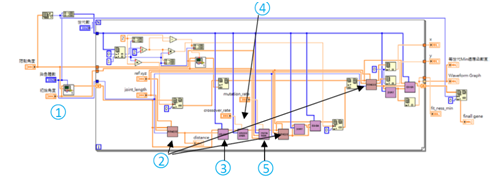
Figure 7 Flowchart of Lab view program based on CUDA.

Figure 8 Schematic diagram for population initialization.
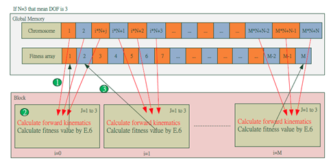
Figure 9 Schematic diagram for calculate the Fitness function.
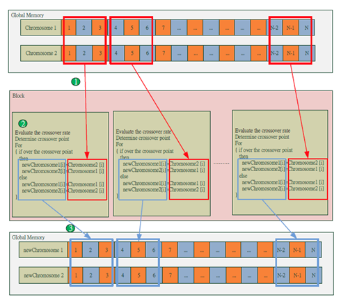
Figure 10 Schematic diagram of crossover operation.

Figure 11 Schematic diagram of mutation operation.

r ¯ 0 = [ x y z ] = A 0 A 1 A 2 A 3 A 4 A 5 A 6 A 7 A 8 r ¯ 8 MathType@MTEF@5@5@+= feaagKart1ev2aaatCvAUfeBSjuyZL2yd9gzLbvyNv2CaerbuLwBLn hiov2DGi1BTfMBaeXatLxBI9gBaerbd9wDYLwzYbItLDharqqtubsr 4rNCHbGeaGqiVCI8FfYJH8YrFfeuY=Hhbbf9v8qqaqFr0xc9pk0xbb a9q8WqFfeaY=biLkVcLq=JHqpepeea0=as0Fb9pgeaYRXxe9vr0=vr 0=vqpWqaaeaabiGaciaacaqabeaadaqaaqaaaOqaaKqbakqadkhaga qeamaaBaaajuaibaGaaGimaaqabaqcfaOaeyypa0ZaamWaaeaafaqa beWabaaabaGaamiEaaqaaiaadMhaaeaacaWG6baaaaGaay5waiaaw2 faaiabg2da9iaadgeadaWgaaqcfasaaiaaicdaaeqaaKqbakaadgea daWgaaqcfasaaiaaigdaaeqaaKqbakaadgeadaWgaaqcfasaaiaaik daaeqaaKqbakaadgeadaWgaaqcfasaaiaaiodaaKqbagqaaiaadgea daWgaaqcfasaaiaaisdaaeqaaKqbakaadgeadaWgaaqcfasaaiaaiw daaeqaaKqbakaadgeadaWgaaqcfasaaiaaiAdaaKqbagqaaiaadgea daWgaaqcfasaaiaaiEdaaeqaaKqbakaadgeadaWgaaqcfasaaiaaiI daaeqaaKqbakqadkhagaqeamaaBaaajuaibaGaaGioaaqabaaaaa@57AF@

Where A i = [ cos ( q i ) cos ( α i ) sin ( q i ) sin ( α i ) sin ( q i ) a 1 cos ( q i ) sin ( q i ) cos ( α i ) cos ( q i ) sin ( α i ) cos ( q i ) a 1 sin ( q i ) 0 sin ( α i ) cos ( α i ) d i 0 0 0 1 ] MathType@MTEF@5@5@+= feaagKart1ev2aaatCvAUfeBSjuyZL2yd9gzLbvyNv2CaerbuLwBLn hiov2DGi1BTfMBaeXatLxBI9gBaerbd9wDYLwzYbItLDharqqtubsr 4rNCHbGeaGqiVCI8FfYJH8YrFfeuY=Hhbbf9v8qqaqFr0xc9pk0xbb a9q8WqFfeaY=biLkVcLq=JHqpepeea0=as0Fb9pgeaYRXxe9vr0=vr 0=vqpWqaaeaabiGaciaacaqabeaadaqaaqaaaOqaaKqbakaadgeada WgaaqcfasaaiaadMgaaKqbagqaaiabg2da9maadmaabaqbaeqabqab aaaaaeaaciGGJbGaai4BaiaacohadaqadaqaaiaadghadaWgaaqcfa saaiaadMgaaKqbagqaaaGaayjkaiaawMcaaaqaaiabgkHiTiGacoga caGGVbGaai4CamaabmaabaGaeqySde2aaSbaaKqbGeaacaWGPbaaju aGbeaaaiaawIcacaGLPaaaciGGZbGaaiyAaiaac6gadaqadaqaaiaa dghadaWgaaqcfasaaiaadMgaaKqbagqaaaGaayjkaiaawMcaaaqaai GacohacaGGPbGaaiOBamaabmaabaGaeqySde2aaSbaaKqbGeaacaWG PbaabeaaaKqbakaawIcacaGLPaaaciGGZbGaaiyAaiaac6gadaqada qaaiaadghadaWgaaqcfasaaiaadMgaaeqaaaqcfaOaayjkaiaawMca aaqaaiaadggadaWgaaqcfasaaiaaigdaaeqaaKqbakGacogacaGGVb Gaai4CamaabmaabaGaamyCamaaBaaajuaibaGaamyAaaqabaaajuaG caGLOaGaayzkaaaabaGaci4CaiaacMgacaGGUbWaaeWaaeaacaWGXb WaaSbaaKqbGeaacaWGPbaajuaGbeaaaiaawIcacaGLPaaaaeaaciGG JbGaai4Baiaacohadaqadaqaaiabeg7aHnaaBaaajuaibaGaamyAaa qabaaajuaGcaGLOaGaayzkaaGaci4yaiaac+gacaGGZbWaaeWaaeaa caWGXbWaaSbaaKqbGeaacaWGPbaabeaaaKqbakaawIcacaGLPaaaae aacqGHsislciGGZbGaaiyAaiaac6gadaqadaqaaiabeg7aHnaaBaaa juaibaGaamyAaaqabaaajuaGcaGLOaGaayzkaaGaci4yaiaac+gaca GGZbWaaeWaaeaacaWGXbWaaSbaaKqbGeaacaWGPbaajuaGbeaaaiaa wIcacaGLPaaaaeaacaWGHbWaaSbaaKqbGeaacaaIXaaabeaajuaGci GGZbGaaiyAaiaac6gadaqadaqaaiaadghadaWgaaqcfasaaiaadMga aKqbagqaaaGaayjkaiaawMcaaaqaaiaaicdaaeaaciGGZbGaaiyAai aac6gadaqadaqaaiabeg7aHnaaBaaajuaibaGaamyAaaqabaaajuaG caGLOaGaayzkaaaabaGaci4yaiaac+gacaGGZbWaaeWaaeaacqaHXo qydaWgaaqcfasaaiaadMgaaKqbagqaaaGaayjkaiaawMcaaaqaaiaa dsgadaWgaaqcfasaaiaadMgaaeqaaaqcfayaaiaaicdaaeaacaaIWa aabaGaaGimaaqaaiaaigdaaaaacaGLBbGaayzxaaaaaa@B0FE@ and r ¯ s = ( 0 , 0 , 20 , 1 ) MathType@MTEF@5@5@+= feaagKart1ev2aaatCvAUfeBSjuyZL2yd9gzLbvyNv2CaerbuLwBLn hiov2DGi1BTfMBaeXatLxBI9gBaerbd9wDYLwzYbItLDharqqtubsr 4rNCHbGeaGqiVCI8FfYJH8YrFfeuY=Hhbbf9v8qqaqFr0xc9pk0xbb a9q8WqFfeaY=biLkVcLq=JHqpepeea0=as0Fb9pgeaYRXxe9vr0=vr 0=vqpWqaaeaabiGaciaacaqabeaadaqaaqaaaOqaaKqbakqadkhaga qeamaaBaaajuaibaGaam4CaaqcfayabaGaeyypa0ZaaeWaaeaacaaI WaGaaiilaiaaicdacaGGSaGaaGOmaiaaicdacaGGSaGaaGymaaGaay jkaiaawMcaaaaa@41A1@ denotes the position of the end effector with respect to the 8th coordinate system and r ¯ 0 MathType@MTEF@5@5@+= feaagKart1ev2aaatCvAUfeBSjuyZL2yd9gzLbvyNv2CaerbuLwBLn hiov2DGi1BTfMBaeXatLxBI9gBaerbd9wDYLwzYbItLDharqqtubsr 4rNCHbGeaGqiVCI8FfYJH8YrFfeuY=Hhbbf9v8qqaqFr0xc9pk0xbb a9q8WqFfeaY=biLkVcLq=JHqpepeea0=as0Fb9pgeaYRXxe9vr0=vr 0=vqpWqaaeaabiGaciaacaqabeaadaqaaqaaaOqaaKqbakqadkhaga qeamaaBaaajuaibaGaaGimaaqabaaaaa@3891@ denotes the position of the end-effector, P0, which is relative to the base coordinate system. The fourth step is to obtain the inverse-kinematic solutions using the proposed EAMP method for the tracking task with the consideration of obstacle avoidance. To compare the computing performance for the serial and parallel RGAMP methods from the perturbation motion planning method,5 the designed parameters of perturbation are described in Table 3. In addition, the results for the CUDA-based EAMP using GPU with the PRNG of the GPU are denoted as CEA. The experimental results for him EAMP using CPU only are denoted as GA. The parameters of GA for the proposed EAMP, which are the crossover rate, mutation rate, generation number, and population number, are also described in Table 3. From Figure 6, the communication needs 4 times to copy data in the crossover and mutation process, because the initial data is needed to copy to GPU from Host and then it is copied from GPU to Host as calculating finished. Therefore, the CUDA EA program is modified to combine crossover and mutation operator as shown in Figure 12 so that the number of copying can reduce to 2 times.

Experimental results and discussions

For the CUDA-based EAMP method, it takes about 48 and 106 seconds for the total computing time of motion planning in the trajectory tracking task with obstacle avoidance (1000 planning points). For each tracking point, the CEA spends 48 and 106 (ms) of computing time for the different GA parameters as shown in Table 4. The computing performance of the proposed CEA (with 48/106 ms) is much faster than the perturbation motion planning method (with 19083 ms). The speed up rate of the CEA is about 398 and 180 with respect to the perturbation method; Figure 13 shows the inverse kinematic solution obtained by the CEA. As shown in Table 4, the GA has the speed up rate of 224 with respect to the perturbation method for the population number of 500 with the generation number of 10. Even the proposed method is implemented on PC only, the computation performance is much better than the past method. Table 4 shows that using the perturbation method cannot achieve the real-time motion planning, because it take a very large computing time, 19.083 seconds per step, for the trajectory tracking with avoidance obstacle cost. However, the proposed CEA/GA methods only need 48/78 (ms) per step for this task-priority task, so that there may be some chance to achieve the real-time motion planning for the redundant robot. To check the priority task of obstacle avoidance, Figure 14 shows the trajectory planning of robot manipulators with free-collision in simulation by open GL and Figure 15 shows the real-time implementation of the 8 DOF robots for the trajectory tracking task with obstacle avoidance. These results show that the proposed method can perform the obstacle avoidance task with keeping the end-effector on the desired trajectory at the same time.

Initial angle of each link

q1=0.0 q2=-90.0 q3=-50.0 q4=0.0 q5=-50.0 q6=0.0

q7=-25.0 q8=0.0 (deg)

Li, Ui

+0.5~-0.5

+0.5~-0.5

+0.5~-0.5

+0.5~-0.5

+0.5~-0.5

+0.5~-0.5

+0.5~-0.5

+0.5~-0.5 (deg)

ni

4

Robot manipulator origin

[0,0,0]

Tracking point

1000

Departure and destination of trajectory

Departure: [17.0, 57.6,30.5]

Destination: [11,110,40]

Obstacle coordination

[15,50,50],[5,50,50],[5,100,50],[15,100,50]

Parameters of GA

Crossover=0.8

Mutation=0.03

Generation=10

Population=500,1000

Terminated condition: generation number

Table 3 Parameters setup for the perturbation method and the RGAMP

Figure 12 Flowchart of the proposed CUDA-based EAmotion planning.

Figure 13 Inverse kinematic solution using the proposed method.

Figure 14 Motion planning simulation of the tracking task with obstacle avoidance.

Population No.

Average Time

Speed up Rate

/Generation No.

(ms/step)

Perturbation method

ni = 4

19083

CEA

500/10

48

398

1000/10

106

180

GA

500/10

78

244

1000/10

152

126

Table 4 Computing time of the three methods

Figure 15 Implementation for the tracking task with obstacle avoidance.

Conclusion

This paper proposed a CUDA- based EAMP method for a robot with 8DOF to track a trajectory with obstacle avoidance. According to the experimental results, the speed up rate for the proposed method is very significant. Moreover, the motion planning methods based on CEA/GA were also studied and the priority task with two main tasks has been achieved. The proposed RGAMP is 398 times faster than the perturbation method for this case study. Finally, experimental results using NI Compact RIO® validate the proposed method feasible for real-time motion planning of the redundant robot.

Acknowledgements

None.

Conflict of interest

The author declares no conflict of interest.

References

  1. Martin BJ, Bobrow JE. Minimum effort motions for open chain manipulators with task-dependent end-effector constraints. Int J Rob Res. 1999;18(2):213–224.
  2. Zhang Y. Inverse‐free computation for infinity‐norm torque minimization of robot manipulators. Mechatronic. 2006;16:177–
  3. Zhang Y, Wang J. A dual neural network for constrained joint torque optimization of kinematically redundant manipulators. IEEE Transactions on Systems, Man, and Cybernetics, Part B (Cybernetics). 2002;32(5):654–
  4. Lin CJ. Motion planning of redundant robots by perturbation method. Mechatronics. 2004;14(3):281–297.
  5. Saravanan R, Ramabalan S, Balamurugan C. Evolutionary collision-free optimal trajectory planning for intelligent robots. Int J Adv Manuf Technol. 2008;36(11):1234–1251.
  6. Maria da Grac Marcosa, JA Tenreiro Machadoa, TP Azevedo‐ A multi‐objective approach for the motion planning of redundant manipulators. Applied Soft Computing. 2012;12:589–599.
  7. Joo H Kim, Chang B Joo. Optimal motion planning of redundant manipulators with controlled task infeasibility. Mechanism and Machine Theory. 2013;64:155–174.
  8. Yoshikawa T. Manipulability of robotic mechanisms. Int J Rob Res. 1985;4(2):3–9.
  9. Karl Lukas Knierim, Oliver Sawodny. Tool-Center-Point control of the KAI manipulator using constrained QP optimization. Mechatronics. 2015;30:85–93.
  10. Lloyd JE, Hayward V. Singularity‐robust trajectory generation. Int J Rob Res. 2001;20(1):38–
  11. Hyejin Han, Jaeheung Park. Robot control near singularity and joint limit using a continuous task transition algorithm. International Journal of Advanced Robotic Systems. 2013;10(10):346.
  12. Lin CJ, Lin CR, Yu SK, et al. Singularity Avoidance for a Redundant Robot Using Fuzzy Motion Planning. Applied Mechanics and Materials. 2014;479‐480:729–736.
  13. Zhang Z, Zhang Y. Variable joint-velocity limits of redundant robot manipulators handled by quadratic programming, IEEE/ASME Transactions on Mechatronics. 2013;18(2):674–686.
  14. Zhang Y, Zhang Z. Repetitive Motion Planning and Control of Redundant Robot Manipulators, Springer Science & Business Media; 2013.
  15. Whitney DE. Resolved motion rate control of manipulators and human prostheses. IEEE Trans Man-Mach Syst. 1969;10:47–53.
  16. Klein CA, Huang CH. Review of pseudo inverse control for use with kinematically redundant manipulators. IEEE Trans Syst Man Cybern. 1983;13(3):245–250.
  17. Baillieul J. Kinematic programming alternatives for redundant manipulators. Proc IEEE Int Conf Robot Automat. 1985. p. 722–728.
  18. Qiu CW, Cao QX, Sun YJ. Redundant Manipulator Control with Constraints for Sub goals. Proc IEEE Int Conf Automat Sci Eng. 2006. p. 212–217.
  19. Saravanan R, Ramabalan S. Evolutionary minimum cost trajectory planning for industrial robots. J Intell Robot Syst. 2008;52(1):45–77.
  20. Pires EJS, Machado JAT, Oliveira PBM. Manipulator trajectory planning using a MOEA. Appl Soft Comput J. 2007;7(3):659–667.
  21. Marcos MG, Machado JAT, Azevedo-Perdicoulis TP. An evolutionary approach for the motion planning of redundant and hyper-redundant manipulators. Nonlinear Dyn. 2010;60(1):115–129.
  22. Satish N, Harris M, Garland M. Designing efficient sorting algorithms for many core GPUs. In Proc. 23rd IEEE International Parallel and Distributed Processing Symoposium; USA: IEEE; 2009.
  23. Liu TS, Tsay SY. Singularity of robotic kinematics: a differential motion approach. Mech Mach Theory. 1990;25(4):439–448.
  24. NVIDIA Fermi Compute Architecture Whitepaper; 2009.
  25. Lin CJ, Chen CS, Yu S K A. GPU-based motion planning for a redundant robot using a parallel genetic algorithm, ICMT Int Conf; Taiwan: IEEE; 2014.
  26. Nakamura Y, Hanafusa H. Inverse kinematic solutions with singularity robustness for robot manipulator control. J Dyn Syst Meas Control. 1986;108(3):163–171.
  27. Maciejewski A, Klein Ch. The singular-value decomposition: computation and application to robots. Int J Rob Res. 1989;8(6):63–79.
  28. Mayorga RV, Janabi-Sharifi F, Wong AKC. A fast approach for the robust trajectory planning of redundant robot manipulators. J Rob Syst. 1995;12(2):147–161.
  29. Holland JH. Adaptation in natural and artificial systems. USA: The University of Michigan Press; 1975.
  30. Rechenberg I. Evolutionsstrategie: optimierung technischer systeme nach Prinzipien der biologischen evolution. Stuttgart: Frommann-Holzboog; 1973.
  31. Nelles O. Nonlinear system identification. Berlin: Springer; 2001.
  32. Langdon WB. Afast high quality pseudo random number generator for nVidia CUDA. Proc 11th Ann Conf Comp Gene & Eol Comp, New York: The ACM digital library is published by the association for computing machinery.; 2009. p. 25511–25514.
  33. Knuth DE. Art of Computer Programming. Volume 2: Seminumerical Algorithms. 3rd ed. USA: Addison-Wesley Longman; 1997.
  34. Matsumoto M, Nishimura T. Mersenne twister: a 623-dimensionally equidistributed uniform pseudo-random number generator. ACM Trans Model Comput Simul. 1998;8(1):3–30.
  35. Marsaglia G. Xorshift RNGs. J Statistical Software. 2003;8(14):1–6.
  36. CUDA Toolkit; 2012.
Creative Commons Attribution License

©2017 Lin, et al. This is an open access article distributed under the terms of the, which permits unrestricted use, distribution, and build upon your work non-commercially.